nueva página del texto (beta)
 Inglés (pdf)
 Artículo en XML
 Referencias del artículo
 Enviar artículo por email
 Citado por SciELO
  Similares en
SciELO
Similares en
SciELO 
 Permalink
1. Introduction
Energy efficiency (EE) is currently on the public agenda worldwide given global warming and the need for energy security for nations. Additionally, given the spread of SARS-COV-2 causing COVID-19, a further call to support sustainable socioeconomic development has been made (IEA, 2020), especially to ensure access to clean and cheap energy in low income and rural households (Barbier and Burgess, 2020). Mexico has been implementing public policies for improving energy usage and production since the 1980s (Economic Commission for Latin America and the Caribbean -ECLAC-, 2018). Its commitment towards greener policies was endorsed with the adoption of the United Nations Agenda 2030 for Sustainable Development.
The adoption of internationally comparable methodologies for energy registers and related data is among the most needed actions to comply with the international agenda in terms of EE because it could inform about the current situation at the country level as well at other administrative levels. The members of the International Energy Agency (IEA), consisting mostly of developed countries, have been producing internationally comparable statistics from late seventies, while Mexico has recently fully adopted the methodology (IEA, 2014). In fact, Mexico joined as a member of the IEA just from February 2018.
Achieving the global goals on greenhouse gas emissions is not possible if larger efforts towards the assessment of EE are not made, which in the case of Mexico is still scarce considering that there are no detailed EE indicators for states, cities or for all sector users, despite the territorial aspect being essential for achieving effective EE public policies (Halkos and Polemis, 2018). This paper contributes to filling this gap by offering an estimation of EE by state, which, to the best of our knowledge, is the first regional EE estimation. Consequently, these estimations can be used for specific regional energy policy design.
We followed the technique proposed by Filipini and Hunt (2011), which consists of the employment of a stochastic production frontier (SPF) model to estimate energy intensity as a proxy for EE. The model estimates the EE for 29 states for the period 1997-2016, and we identified three variables as sources of energy inefficiency. Considering the ECLAC (2018) analysis, our results are in line with the estimations at the country level, namely, we confirmed that EE has increased in the period of study, but in addition, we provide state-level estimations. One limitation of the work is that due the lack of data availability, the model only includes electricity as the total primary energy supply, leaving out other important sources such as gasoline and diesel. Therefore, the estimation relates only to EE in electricity usage, in which intensive sector users are the industrial, residential and services, and, to a lesser extent, agricultural (SENER, 2018).
The EE in the use of electricity is particularly important in Mexico because most public policies aiming at increasing EE over the last 30 years have been focused to diminish electricity consumption of residential and industrial sector users by promoting the usage of more efficient electronic devices, the substitution of incandescent light bulbs, and the use of solar powered devices for water heating and lighting (ECLAC, 2018).
The structure of the paper is divided into five sections. The first section shows this introduction. The second section discusses the current state and studies about EE in Mexico. In the third section, the method and data used in our estimations are depicted. In the fourth section the results are presented and discussed. The fifth section presents conclusions and policy implications.
2. Energy Efficiency in Mexico
2.1 What is Energy Efficiency?
The use of energy intensity (EI) indicators as a proxy for EE is very common, given that these concepts are highly related and that the former is easier to estimate, despite the definition of the latter being easier to grasp. According to IEA (2014), defining these indicators can be difficult, but as a matter of fact, the concept of energy efficiency is easier to understand: “energy efficiency is using less energy to provide the same service” (IEA, 2014; p.17). Meanwhile, evaluating directly if something is being more energy efficient is not simple considering that several factors can change the demand of energy; for instance, users started using another energy source to provide the same service.
Energy intensity is the ratio between the total primary energy supply by the gross domestic product (GDP), which can be estimated at the country, sector, or even firm level, and it can be determined by the climate, infrastructure, culture and technology employed in the production process (IEA, 2014). The data for its estimation are easily available; thus, EI is the most commonly used indicator for assessing EE. For the estimation of EE, instead, the energy consumption and activity data are employed. Energy consumption can be expressed in several units (kWh, joules, tons of oil, etc.) while activity data, is what the energy is used for, such as, lighting, water heating, transporting passengers, and others. In addition, sector/end-users are also taken into account for sector estimations to produce detailed indicators by providing data on specific sectors, such as transport, residential, manufacturing, services and agricultural Namely, considering a dwelling demanding electricity for lighting, an EE indicator can be estimated as kWh for lighting a dwelling. In such cases, the user can be a household (residential) or a firm (services); the source of energy supply is electricity, and the activity data are lighting. Likewise, the same dwelling can use electricity for cooking, water heating, cooling/illuminating spaces, etc.; in such cases, the user and energy source remain unchanged, while the activity data are different in every case. In sum, EI indicators use value added or production as activity data, while EE indicators employ many different activity data depending on the purpose of the energy used.
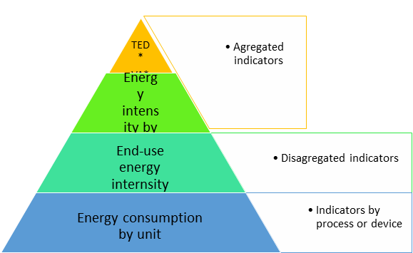
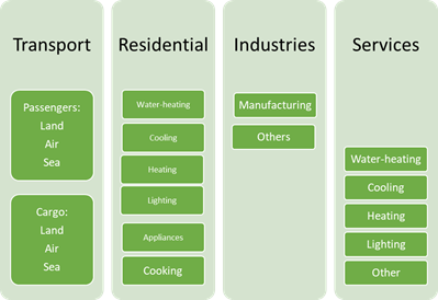
In illustration 1, the sector users or end-users are shown as well as their main activity data-aims-of usage. The end users can also be grouped differently across countries; in Mexico, the sector users are Industrial, Transport, Residential and services, and Agricultural, Residential and Services are grouped together given that the end-uses are almost the same. Regarding energy sources, they can vary between countries depending on their availability or price; for instance, in some countries, it is common to use natural gas for heating, while in others, it is more frequent to use electricity; consequently, different energy sources are employed for similar activities around the world (IEA, 2017).
EE indicators can be estimated at the macro or micro level; in any case, the estimations require a large amount of information, such as the total primary energy supply, sector users and activity data (aim/end-use). The aggregate indicator with the largest scope is at country level, yet even at this level, it is necessary to produce the registers of all energy sources, sector users and the aim of usage. At the aggregate level, EI is frequently estimated using the sum of all types of energy sources divided by the total GDP in the country (IEA, 2014). Micro indicators could be very detailed, referring to a firm, a device, or a household, with specific activity data, such as the amount of natural gas for heating 40m2 construction in a dwelling or liters of diesel to transport a passenger by plane divided by kilometers transported. The levels of aggregation are shown in illustration 1 in the annex; for more detailed information, please consult (IEA, 2014).
The micro indicators require a larger amount of information, which is obtained from administrative registers and usually complemented by surveys. Nevertheless, collecting the information is a complex process, and there are indeed some sectors in which the collection is even more difficult, such as in agricultural activities and those using alternative sources of energy (IEA, 2014). The most accurate method to obtain data is surveying; however, it is costly and time consuming. According to the IEA, an affordable approach for estimating EE indicators is the usage of statistical models, which helps to build indicators when all the other options are not possible (IEA, 2014), even though these indicators are less accurate than those estimated with other techniques.
2.2 Where is Mexico in Energy Efficiency?
The first project to measure EE in Mexico started in 2008, with financial and technical support from the IEA and the United Kingdom (UK) (SENER and IEA, 2011), and the results were published until 2015. The indicators only included three sectors: schools (SENER, 2015a), hotels (SENER, 2015b) and hospitals (SENER, 2015c) but with a limited chosen sample. The most recent and complete publication about EE in Mexico is ECLAC (2018), which presents an analysis of the evolution of energy intensity and sources of energy supply for all sector users, such as manufacturing, transport, services, residential, agriculture and fishery. The results showed only energy intensity, which only takes the total energy input divided by the value added as activity data. However, regional estimations at the state or municipality level cannot be done given the lack of specific information by sources and end-users at state and municipality level in Mexico. Consequently, statistical estimations are the only way to proxy EE by state in Mexico.
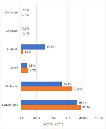
Even if the estimations of EE in Mexico are still scarce, the harmonization of registers, the adherence of the country to the IEA and the slight reduction of oil-based energy sources are proof of the progress in the subject. Indeed, producing standardized data for international comparison requires great effort (IEA, 2018). Additionally, according to the ECLAC (2018), Mexico has reduced its dependence on oil-based fuels by means of incentivising the use of natural gas. Namely, in 1990, 55.4% of the total energy used came from oil-based fuels and 29.9% from natural gas; by 2015, the proportions shifted to 40.5% and 44.3%, respectively. In addition, the increment of electricity usage within the last 20 years is significant, and within this period, electricity became the second most important fuel. For instance, in 2000, the shares of energy demand by fuel were gasoline 26%, diesel 15%, and electricity 15%; by 2015, the shares changed as follows: gasoline 30%, electricity 17.3% and diesel 17.1%. It is necessary to remark that the major sector users of electricity in Mexico are the industrial and residential sectors and services, as shown in illustration 2.
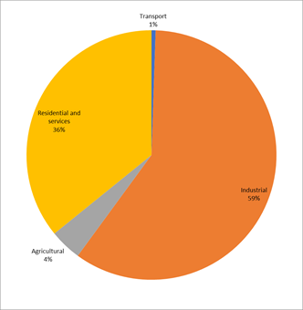
Source: Own elaboration with data from ECLAC (2018)
Illustration 2 Share of electricity consumption by sector, 2015
It is also worth noting that in recent years, the energy sources for both industrial and residential services have diversified. Certainly, the ranking by importance of energy sources for all users-sectors shifted between 2000 and 2015. This is shown in illustration 3.
Source: Own elaboration with data from ECLAC (2018)
Illustration 3 Energy sources for Industrial sector user
Considering these changes in the total energy supply by type of energy, as seen in the energy matrix, the ECLAC has rated the Mexican policies as successful mainly due to the decreased dependence from oil-based fuels. Specifically, policies have been addressed towards the reduction of oil-based fuels and the promotion of new device usages, which use cleaner energy sources and are more energy efficient. In the case of the residential and industrial sectors, the most important actions are the substitution of incandescent light bulbs and the usage of solar powered devices for water heating and lighting. Derived from these policies as well as influenced by other factors, the EI showed a reduction of 45.9% in the residential sector and 15.6% in the industrial sector during the period 1995-2015.
Furthermore, in early 1990, the national standards for EE came into force (NOM-ENER), which aimed at promoting greater EE in end-users rather than in energy producers. However, the electricity supplier, a state-owned company, the National Electricity Commission (CFE by Spanish acronym) during the 1990s and until 2005, had increased its demand for natural gas, substituting coal and fuel oil for electricity production. This led to the decrease in EI (improvement of EE). Yet in 2005, the demand of coal and fuel increased again due to high costs of natural gas. Nevertheless, after the 2009 crisis, the energy intensity has reduced significantly as a result of various facts, in addition to the public policies implemented. Namely, ECLAC (2018) highlights that the tertiarization of the economy and technology innovations have also influenced the reduction of EI. Nonetheless, even if there have been significant improvements in EE in recent years, Mexico is far from the international trend (Sandoval, Matsumoto and Pedraza, 2020).
3. Materials and methods
3.1 Stochastic Production Frontier Analysis
This model is based on the microeconomic concept of the production frontier, operationalised as a statistical model initially by Aigner, Lovell and Schmidt (1977). It is based on the idea that a company, in this case a region, has certain production factors, from which if it optimises their use, that will allow the firm to reach a given level of production. The border function will provide the maximum output level or the minimum feasible cost for the production entity. However, not all companies or entities ought to reach the same level of production/costs, even if they employ the same production inputs, suggesting that some firms/regions are more inefficient than others. The inefficiency can be either unobservable and considered as a result of a random process or observable and taken as the result of a set of variables.
SPF is frequently used to estimate efficiency or inefficiency. The empirical application has basically followed two approaches: a parametric approach and a non-parametric approach. The first is based on econometric techniques, and the second is based on mathematical techniques such as data envelopment analysis (DEA) (Ali et al. 2019).
The parametric approach, commonly called the stochastic production frontier model, has been applied to estimate technical efficiency in companies, producers and regions, e.g., in the agricultural sector of different countries such as India (Ali and Gupta, 2011), China (Wang and Rungsuriyawiboon, 2010), South Africa (Pauw, McDonalds and Punt, 2007), and Mexico (Becerra-Perez, Lopez-Reyes and Tyner, 2017). The main advantage of the SPF model is that it separates the random error from the inefficiency effect. The nonparametric approach estimates an error term accounting for random and other potential sources of inefficiency that cannot be explained by exogenous variables (Ali et al., 2019), while the SPF model estimates a two-part error term, a random term and a not random term, which can be explained by other variables causing inefficiencies.
The same definition is applied to the energy demand function in a state, that is, when goods and services are produced, the difference between the observed energy demand by a state and the minimum energy demand may be caused by inefficiencies determined by one or more variables. In the case of the aggregate energy demand function used here, the frontier provides the optimal energy demand. In other words, the estimation of the boundary function for energy demand allows us to estimate a reference energy demand that is optimal. This border approach permits assessing whether a given state is located on the border; if not, the distance from the border is an indicator of energy inefficiency (Otsuka and Goto, 2015).
In this empirical application, the methodology used by Otsuka et al. (2015), initially proposed by Filippini and Hunt (2011), is employed to estimate an energy efficiency indicator for the entire economy using panel data. Filippini et al. (2011) proposed a model that measures energy efficiency through an energy intensity indicator, which is the total primary energy used divided by the GDP for OECD countries. Otsuka et al. (2015) estimated the energy intensity at the regional level for 47 prefectures in Japan, assuming that there is an aggregate energy demand function at the prefectural level in Japan, as shown below.
The subscript j represents the j-th region, and t represents the t-th period. E is the final energy consumption, Y is the real gross regional product (GRP), P is the real price of energy, POP is the population, and DCF and DCC are cold weather days and warm weather days, respectively. PIM and PS represent the share of manufacturing and services from the total GRP, respectively. EE is the level of underlying energy efficiency not observable.
The underlying energy efficiency includes the effects of several factors that vary across regions. An example of this may be institutional frameworks, differences in social environments and economic structure as well as differences in culture, lifestyle, and values. Here, when the underlying EE is small, it means that there is a waste of energy; on the contrary, a large EE shows energy savings, with a given level of GRP.
As pointed out by the International Energy Agency, the estimation of energy efficiency requires disaggregated indicators that are difficult to obtain and are often not available. Hence, aggregate indicators are often used for the study of energy efficiency (IEA, 2014); nonetheless, aggregate indicators cannot explain the underlying EE; thus, it must be modelled through a statistical model.
Stochastic frontier models for panel data were initially proposed by Pitt and Lee (1981), yet that estimator did not allow adding exogenous explanatory variables for the inefficiency term. Later, the estimator proposed by Greene (2005) allows estimating fixed effects for panel data, and the invariant inefficiency derived from the characteristics of each region can also be estimated through the time. A further advantage of using Greene’s estimator is that the inefficiency term can be heteroscedastic. Consequently, we used this estimation method to control for fixed effects while allowing differences across regions. Notwithstanding, there are additional assumptions about the distribution of the inefficiency term, which led to the model being criticized. In response, Belotti and Ilardi (2018) proposed different developments to improve the estimations. However, it was not yet available for its estimation in the software used. Consequently, we used the estimation method proposed by Greene (2005) using the true fixed effects (TFE). We employed Stata for the estimations because it permits the performance of diverse tests and estimation options; for further details, it is advisable to review Belotti, Daidone, Ilardi and Atella (2013).
The model was estimated in levels using natural logarithms of all variables. The baseline equation is defined as follows:
The dependent variable E jt is the total electricity consumption of state j in year t. α j represents an estimated parameter for each state j. Y jt corresponds to the added value of state j in year t. P jt is the average price of electric power in state j in year t. POP jt is the population of state j in year t. CDC jt and CDH jt are the climatic differences for cold and warm days, respectively, compared with the national average, by state j in year t, which were calculated as cumulative differentials. In Mexico, the use of cooling equipment in all sectors is more common than heating, so the CDH variable is expected to have a greater effect on energy demand. In fact, for states registering higher temperatures during summertime, the federal government grants a subsidy to the price of electricity, given the high levels of consumption in all sector users. PIM jt and PS jt are the share of manufacturing and services industries from the total gross production in state j in year t.
The error term is composed of two parts
Following Otsuka et al. (2015), energy efficiency can improve given certain conditions in the regions; the most important factors are population density, access to markets, and the presence of industries with high levels of energy requirements, which, according to IEA (2014), correspond to materials industries. Materials industries are considered wasteful given that they demand great amounts of energy to produce a monetary output of value added; in other words, they show a high EI in comparison to other industries. Our model includes the same variables used by Otsuka et al. (2015) as the exogenous determinants for the underlying energy inefficiency:
where α is the constant parameter. Dens it is the population density (total population/state area in km2) in state i in year t. PM it is the market potential of state i in year t. MatInd it is the share of the materials industry as compared to the total manufacturing for state i in year t. To interpret the sign of the coefficients in this equation, it is necessary to bear in mind that the underlying inefficiency is measuring the waste; thus, a variable increasing energy waste would show a positive sign, while the opposite is expected for variables decreasing energy waste. In this manner, when the energy inefficiency ϵ it is improved due to one exogenous variable in equation 4, the corresponding βn should be negative. The MP variable proposed by Ibarra-Armenta (2018) was used, which estimates the market potential for all Mexican states considering adjacent regions within a radius of 350 km. This radius is estimated from the capital city of each state to all the other capital cities in the country. Of course, there are firms that produce only one plant and distribute their products all around the country regardless of their geographic location, and therefore, the potential market might be larger; nonetheless, we are considering that for most firms, their commercialization boundaries are contained within a certain geographic range. Materials industries correspond specifically to the chemical, paper and pulp, iron and steel, non-ferrous metals, and cement industries, which have been identified as high energy consumers per unit of added value produced, according to IEA and Filippini et al. (2011). We do not have the specific data to test this assumption, but we supposed that in Mexico, these industries observe similar behaviour to the OECD average; that is, those industries have greater energy intensity compared to other manufacturing industries (Filippini et al., 2011).
Earlier results confirmed that cities with low population density may be less energy efficient; therefore, EE could improve if the city were more compact, i.e., with greater population density (Otsuka et al., 2015). Hence, it is expected that EE increases as population density increases; in such cases, the corresponding β coefficient should have a negative sign because it reduces the energy waste. Market potential can affect EE because isolated regions need to spend more energy for trading, especially in regions with poor highway communication systems. For instance, if the travel time to other regions is reduced through the improvement of the road network, energy efficiency could also be improved. Thus, MP is expected to also show a negative sign because a greater MP reduces EI and thus increases EE. In sum, whether these assumptions are valid, the β coefficients of Dens and MP are expected to show a negative sign. On the other hand, given that the materials industries are expected to show high EI, MatIn is expected to increase energy inefficiency; therefore, its β coefficient is expected to be positive.
3.2 Data
Various sources of information were consulted to obtain the data used. The data on energy consumption and energy prices were taken from the Ministry of Energy (SENER by Spanish acronym) database. Production variables as well as geographic data were obtained from the National Institute of Statistics and Geography (INEGI by Spanish acronym). Population data were obtained from the National Council for Population (CONAPO by Spanish acronym); specifically, the dataset used is the population projections by state until 2030. Climate data were obtained from databases of the national meteorological system.
Two states, Estado de Mexico and Hidalgo in the centre region of the country, did not have complete information for the chosen period; thus, they were extracted from the sample. The estimation period is 1997-2016 due to data availability on energy consumption per state from SENER.
Table 1 shows the statistical summary of the variables included in the model.
Table 1 Summary statistics
| Variable | Mean | Standard error | Min | Max |
|---|---|---|---|---|
| Energy Consumption (Gigawatts/hour) | 5,276.71 | 3,992.86 | 245.32 | 18,609.54 |
| Population | 3,427,340 | 2,863,102 | 396,454 | 17,118,525 |
| Climatic Difference from National Average (Heat) | 93.61 | 40.96 | 15.00 | 182.00 |
| Climatic Difference from National Average (Cold) | -58.79 | 64.89 | -167.00 | 74.00 |
| Share of Manufacturing | 17.51% | 11.69 | 0.27% | 64.43% |
| Share of Services | 61.34% | 14.30 | 7.57% | 93.79% |
| GDP (MXN Constant prices 2013) | $412,677 | $440,954 | $60,159 | $2,974,070 |
| Average Price of Electricity (MXN Constant prices 2013) | $145 | $ 39 | $ 97 | $222 |
| Market Potential (MXN Constant prices 2013) | $428,020 | $446,155 | $61,579 | $3,041,181 |
| Share of Material Industries from total manufacturing | 10.60% | 14.68% | 0.79% | 85.58% |
| Population Density (Inhabitants/km2) | 275.51 | 1,052.07 | 5.36 | 6,021.31 |
Source: Own elaboration
4. Results and discussion
Considering that this is a log-log model, the coefficients represent the elasticity of each of the variables with respect to energy consumption. The estimation results are shown in table 2. Given the demand drivers highlighted by the IEA (2014), it was sensible to expect that variables such as the value added (Y jt ) and population (POP jt ) were statistically significant given that population and production raises may increase the demand for electricity. Nonetheless, both variables were not statistically significant.
The variables observing an important effect on energy demand are the economic structure and the climate. For the latter, it is clear that a warm climate has a greater effect on energy consumption than a cold climate. For instance, states with warmer climates show an increase in demand of 0.17% by a 1% increase in the temperature difference compared to the national average, while the elasticity for cold climate is only 0.0009%. Regarding the economic structure, both manufacturing and services showed elasticities of similar size; 1% growth in the share of these industries showed 0.25% and 0.23% increases in energy demand, respectively.
Table 2 Estimation results
| Dependent Variable: ln Electricity Consumption | (1) |
| Ln Population (inhabitants) | 0.1017 |
| (0.1394) | |
| Ln Climate Difference for Hot weather | 0.1702*** |
| (0.0444) | |
| Ln Climate Difference for Cold weather | 0.0009** |
| (0.0004) | |
| Ln Manufacturing share | 0.2521*** |
| (0.0469) | |
| Ln Services share | 0.2338*** |
| (0.0806) | |
| Ln Y (constant prices 2013) | 0.0986 |
| (0.0810) | |
| Ln Average Price (constant prices 2013) | 0.3687*** |
| (0.0707) | |
| u ij | |
| Ln Market Potential (Constant prices 2013) | -0.2396*** |
| (0.0608) | |
| Ln Material Industries Share (from total manufacturing) | 0.2642** |
| (0.1104) | |
| Ln Population Density (inhab/km2) | -0.8550*** |
| (0.1936) | |
| _cons | 1.6843 |
| Vsigma | |
| _cons | -5.7533*** |
| (0.3773) | |
| Sigma_v | 0.0563 |
| (0.0106) | |
| N | 600 |
| Standard errors in parenthesis *0.1, **0.05, ***0.01 *0.10, **0.05, ***0.001 |
Source: Own elaboration with estimations results
In microeconomic theory, the price of normal goods are expected to show a negative relation with the demand function; however, Thollander, Danestig and Rohdin (2007) claim that given the importance of energy, its demand tends to be inelastic; hence, the price does not deter its consumption, and other policies should be followed to achieve savings in the long term (Backlund, Thollander, Palm and Ottosson, 2012). The estimations’ results show a positive and statistically significant coefficient; hence, electricity demand is not discouraged by the price, yet the positive sign might be a result of the price strategy implemented by CFE. The rates are scaled depending on the consumption level to encourage energy savings. Namely, CFE sets consumption thresholds with corresponding rates. Low-consumption users pay the lowest price rate. After crossing the first threshold consumers start paying a higher rate and this pattern continues for each successive threshold. Namely, CFE sets consumption thresholds and their corresponding rates, low-consumption users pay the lowest price rate, and after the first consumption limit, the consumer pays the next rate, and so on. Therefore, larger consumption is directly related to higher prices. In addition, as explained before, during summertime, electricity consumption increases considerably in states with hot weather; therefore, a subsidy for all users is given by CFE, which can go up to 50%. Regarding public policy implications, it is necessary to keep encouraging the replacement of equipment and appliances for more energy efficient ones as well as to implement energy management to ensure optimal production conditions for to keep the increasing EE in the long term, which requires continuous work (Backlund et al., 2012).
Concerning the inefficiency term, it is observed that the independent explanatory variables showed the expected signs and are statistically significant. In this way, it is confirmed that the states with larger population density and market potential were more efficient on electricity consumption; in other words, the size of the inefficiency term is smaller when these variables are greater. The coefficient size shows that population density, 0.855%, is the most important driver for the inefficiency term. Meanwhile, the presence of materials industries is positively related to the inefficiency term; that is, a greater presence of material industries fosters energy waste, as predicted.
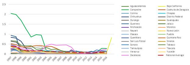
Given that population density is the most important driver for energy inefficiency in our model, illustrations 4 and 5 show the population density by state for 1997 and 2016, respectively.
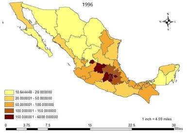
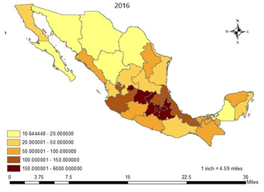
It is clear that the central area of Mexico is the most densely populated, particularly Mexico City and its metropolitan area. It can also be noticed that the states with the lowest population density are within the northern part of the territory, as well as in the southern area.
From the model estimations, the values of energy inefficiency per state were obtained, which are shown in Table 3. It also includes the density ranges in the last column, which helps to relate the map to the ranking in the table. Additionally, a graph of inefficiency values per state for the whole period is included in illustration 2 of the annexes.
Table 3 Energy Efficiency Rank of Mexico State and Growth Rate of 1997-2016
| Mexico State | Rank EE |
Mean EI |
Min | Max |
Growth Rate EI,1997-2016 |
Population Density level 2016 |
|---|---|---|---|---|---|---|
| D. F. (CDMX) | 1 | 0.01319 | 0.0071 | 0.03532 | -72% | 5 |
| Veracruz | 2 | 0.05667 | 0.02889 | 0.08429 | 43% | 4 |
| Tlaxcala | 3 | 0.05792 | 0.02023 | 0.13611 | -71% | 5 |
| Jalisco | 4 | 0.06476 | 0.0169 | 0.11193 | 245% | 4 |
| Puebla | 5 | 0.06733 | 0.02137 | 0.24789 | -91% | 5 |
| Baja California | 6 | 0.06795 | 0.03092 | 0.12182 | 121% | 2 |
| Morelos | 7 | 0.07172 | 0.02412 | 0.37467 | -91% | 5 |
| Tamaulipas | 8 | 0.07549 | 0.0379 | 0.18678 | -61% | 2 |
| Aguascalientes | 9 | 0.07616 | 0.01818 | 0.29503 | -92% | 5 |
| Guanajuato | 10 | 0.07864 | 0.01717 | 0.22292 | -90% | 5 |
| Querétaro | 11 | 0.07884 | 0.02288 | 0.27543 | -92% | 5 |
| Nuevo León | 12 | 0.08595 | 0.02389 | 0.25884 | -87% | 3 |
| Colima | 13 | 0.08891 | 0.02501 | 0.25125 | -81% | 4 |
| Yucatán | 14 | 0.09048 | 0.02957 | 0.30852 | -90% | 3 |
| San Luis Potosí | 15 | 0.09222 | 0.03048 | 0.23834 | -87% | 2 |
| Oaxaca | 16 | 0.09686 | 0.02431 | 0.22709 | -89% | 2 |
| Coahuila | 17 | 0.10526 | 0.02801 | 0.20686 | -33% | 1 |
| Sonora | 18 | 0.10634 | 0.04295 | 0.25734 | -41% | 1 |
| Sinaloa | 19 | 0.11097 | 0.02496 | 0.36935 | -93% | 3 |
| Chiapas | 20 | 0.11844 | 0.01771 | 0.30997 | -94% | 3 |
| Michoacán | 21 | 0.12398 | 0.02102 | 0.45257 | -71% | 3 |
| National Average | 0.13455 | 0.05677 | 0.39334 | -85% | ||
| Guerrero | 22 | 0.15204 | 0.02779 | 0.93639 | -95% | 3 |
| Durango | 23 | 0.17346 | 0.03003 | 0.64268 | -95% | 1 |
| Nayarit | 24 | 0.19207 | 0.0217 | 0.54243 | -96% | 2 |
| Chihuahua | 25 | 0.19379 | 0.03887 | 0.83821 | -95% | 1 |
| Tabasco | 26 | 0.22759 | 0.01915 | 0.67336 | -96% | 3 |
| Quintana Roo | 27 | 0.23562 | 0.01661 | 0.50488 | -97% | 2 |
| Zacatecas | 28 | 0.24539 | 0.02545 | 0.4945 | 0.30% | 2 |
| Baja California Sur | 29 | 0.32764 | 0.03218 | 0.81718 | -96% | 1 |
| Campeche | 30 | 0.56075 | 0.0407 | 2.04316 | -86% | 1 |
Notes: EE = Energy Efficiency; EI = Energy Inefficiency; a negative value in the growth rate of EI means an increase in EE
Source: Own elaboration
Provided that these are inefficiency levels, the smallest value belongs to the most “most efficient” (least inefficient) state. Negative growth rates indicate inefficiency level reductions, which are improvements in EE. Our results are in line with the aggregated estimation from SENER (ECLAC, 2018) since our model showed an improvement of EE for the national average. Nonetheless, when breaking to regions, Veracruz, Jalisco, and Baja California experienced increases in energy inefficiency, although they are still placed among the 10 most efficient regions on national level.
Tabasco and Campeche showed large levels of inefficiency, partially attributed to the large presence of materials industries, which on average represented up to 85% of their manufacturing sector. In addition, their relatively small market potential and low population also contributed to the high inefficiency. Baja California Sur is the state with the lowest population density, which explains its results.
In summary, the model confirmed improvements in EE at the national level while characterizing the performance per state. Moreover, the model confirmed that, similar to other countries, there are exogenous variables related to EE, and therefore, the results can be used for regional public policy design. Namely, first, considering that population density is the larger driver for energy inefficiency reductions, it is important to increase policy efforts towards states/regions with lower densities. Second, given that the centre region benefits from its greater market potential derived from higher population density as well as its high-income level, public policies should address states with smaller market potential which are distant from big markets. Third, it is equally important to design specific policy actions for states with a large presence of material industries to increase the sustainability of such industries.
4.1. Further discussion: Households, the key for climate change
Undoubtedly, more policy actions are needed to achieve a larger reduction in greenhouse gas emissions. According to Dubois et al. (2019), households are the key sector for climate change, considering that they account for 72% of global greenhouse gas emissions. This includes not only the energy demand by end-users but also the demand for goods and services. For instance, in their study, Dubois et al. identified three main components to be addressed: mobility (car and planes), meat and dairy consumption and heating. Additionally, they found that households’ behavior is highly determined by age, health conditions and income. Mobility is particularly significant considering the large increments of private cars from 2000-2015, mainly due to real income increases and poor public transport services (ECLAC, 2018). Thus, it would also be necessary to implement policies boosting the change of behavior from families while managing such actions according to the household’s characteristics.
However, the recent publication by SENER (2018) shows that, in Mexico, the policies implemented to achieve electricity consumption reduction in the residential and industrial sector have only focused on enhancing the change of electronic appliances used for water heating, lighting, cooling spaces, cooking and similar activities. Nonetheless, there is no specific policy to encourage the reduction of the consumption of meat and dairy products or to entail significant changes in mobility habits. Furthermore, the policies are not yet targeted by age, income or other socioeconomic characteristics, which, according to Dubois et al. (2019), would be needed.
In addition, according to ECLAC (2018), during the most recent economic crises in Mexico, 1993 and 2009, EI increased. In fact, Andreoni (2020) showed that among 18 European countries, those hit harder by the 2008 crisis showed higher EE losses than those with greater GDP increases after the crisis. The reasons explaining this trend are indeed an open debate in the empirical and theoretical literature (Andreoni, 2020); one reason could be technical efficiency losses during economic crises, meanwhile the economy tends to gain technical efficiency in economic expansions (Kapelko and Oude Lansink, 2015). Another factor could be that during the economic crisis, the budget for cleaner energy sources is diminished (Andreoni, 2020). Thus, considering the huge economic shock caused by the current sanitary emergency, it is important to pay special attention to the EI during and after the pandemic because EE could also decrease due to the COVID-19 crisis, as occurred before in 1993 and 2009.
The IEA (2020) highlights that even though carbon emissions are expected to diminish as a result of the great reduction in transport demand, a rebound can also occur, as occurred earlier in 2008. In addition, before the pandemic, only a few sectors were on track to achieve long-term sustainable goals. As a result of the huge economic disruption and budget pressions for governments, it is likely that most governments will reduce their investments to achieve the agreed goals.
5. Conclusions, recommendations and final considerations
This work is a pioneer in ranking EE levels of Mexican states. We found that EE on electricity consumption has improved at the national level, in line with the ECLAC (2018) findings. Three variables were identified as common drivers for EE, namely, population density, material industry presence and market potential, with special remarks on the former. Considering these findings, some policy recommendations can be drafted. Given that most densely populated states are more energy efficient, it is important to focus policy efforts towards states with lower population density. Additionally, special attention should be drawn to Tabasco and Campeche given the large presence of materials industries. Regarding market potential, again, given the geographic location, states in the centre and west-centre regions are the ones with larger market potential; hence, perhaps population density is the best reference for policy design. Furthermore, special policy actions should be proposed for those states in which inefficiencies increased, namely, Jalisco, Veracruz and Tabasco, as well as for those showing less improvement throughout the period.
The model showed that electricity prices are positively related to the consumption level. Thus, the current scaled price system does not incentivise users to reduce their electricity consumption, which must be considered for public policy design. Moreover, policy makes need to continue in encouraging the use of more energy efficient equipment and appliances to achieve further reductions of EE. Furthermore, considering studies in other countries, it is necessary to widen the policies implemented to influence the consumption patterns of households in themes such as mobility and meat and dairy product demand. More importantly, detailed policies according to household features would also help to continue reducing energy intensity in the residential sector.
Finally, the COVID-19 crisis could result in increases in energy intensity and reduction of public investment to attaint long-term sustainable goals. In this context, our results become more important as we highlighted variables to incorporate territorial factors into EE policies, which could increase their effectiveness, as highlighted by Halkos and Polemis (2018).