


 nueva página del texto (beta)
 Inglés (pdf)
 Artículo en XML
 Referencias del artículo
 Enviar artículo por email
 Citado por SciELO
  Similares en
SciELO
Similares en
SciELO 
 Permalink
1. Introduction
In late 2019 and early 2020, the oil price war between Russia and Saudi Arabia -one of the member countries of the Organization of the Petroleum Exporting Countries (OPEC)- had a distorting effect on oil production and price. Russia rejected the protectionist agreements of OPEC and declined to cut its production while Saudi Arabia wanted to trade at preferred prices for certain markets. At the same time, the Coronavirus pandemic triggered a slump in oil’s demand. Both effects shook the stock exchanges of several countries.
The production cut, Saudi-Russian price war, and the COVID-19 pandemic propagation around the world began a series of high volatility in the stock market. At the same time, real interest rates started to fall, and growth expectations for advanced and emerging countries plummeted for 2020 and 2021, ranging from -2% to -8% (IMF, 2020). Furthermore, growth forecasts affected credit ratings of the industry and the sovereign debt in most countries.
Risk is inherent in the future, and financial markets must be positioned to face it. These effects can trigger unpredictable, high-impact catastrophes if not managed correctly but, in turn, creates many opportunities in the stock and derivatives market (Bolton, Despres, da Silva, Samama, & Svartzman, 2020). In that sense, it is essential to find financial assets that can be profitable in volatile scenarios and know leading indicators about energy trends, specifically, over oil prices. For that reason, the leveraged energy Exchanged Traded Fund (ETF) is proposed in this analysis.
ETFs can be used as short-term investment instruments and have the main advantage of being linked to any underlying asset, industry, or sector. In this case, bull (upwards) and bear (downwards) ETF are selected yet had one peculiarity: leveraged ETF is focused on speculators seeking to profit in daily trading. Nevertheless, if dynamic risk-return analysis of this ETF is made, it's possible to identify the more profitable leveraged ETF and take advantage of volatility even when energy prices are falling.
This research aims to capture the risk-performance exposure of 4 of the most popular leveraged energy ETFs: GUSH, DRIP, DGAZ, and UGAZ, which are an attractive investment option when the capital market (shares and bonds specifically) do not perform well due to the inherent uncertainty of the market. These instruments are leading indicators of energy prices and commodities (because the composition of ETFs considers these elements). They may be used as possible hedges to address sharp fluctuations in oil and natural gas prices in the current pandemic context.
The research tries to capture two scenarios, yearly and monthly; traditional risk measures independent of the spirit to which traders are exposed when buying and selling instruments. This analysis is relevant to eventually form an expectation over time about volatile energy price behavior, particularly the ETFs that capture this behavior, but not pretend to explain the best scenario to invert.
The next section presents a brief review of risk-return trade-off models, including the Capital Asset Pricing Model (CAPM), which is suitable for obtaining the market beta (β). In section 3, the relevance of acquiring ETFs within the investment portfolio is discussed for those agents who have a greater tolerance for risk, to obtain higher profits than it entails within the investment strategy. Furthermore, we make an exposition of the qualities of the most recognized energy-leveraged ETFs: GUSH, DRIP, DGAZ, and UGAZ as instruments that allow the benefit of the trajectory of the index to which they are referred.
In section 4, we compute a rolling window mean-standard deviation model applied to the leveraged energy ETFs is performed, where volatility, expected return and market beta (β) are estimated in different time horizons for making the investment decision. The implementation allows considering investment profiles for annual and monthly operations. Market beta is set against the S&P500 market index and Chicago Options Volatility Index (VIX).
The results allow characterizing the dynamics of risk-return of bull and bear leveraged energy ETFs and propose a more accurate measure for risk compensation. Except for DRIP, the ETFs exhibited high-beta rolling sensibility to S&P500 and from 0 to 1 for VIX. For those investors who decided to turn to watch and buy these energy instruments, undoubtedly, they took a remarkably high profit or stratospheric losses.
2. Brief Review ff the Risk-Return Trade-Off
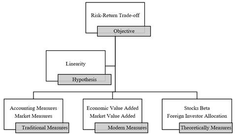
The financial sector requires new models to operate adequate risk management because of market developments, new technologies, and a wide range of financial and derivative products. One of the most used methods for calculating the inherent risk of a project is the risk-return trade-off (Ye & Tiong, 2000). This method is an estimate of the expected risk and thereby capture the minimum compensation required to accept the level of risk exposure (Manotas-Duque & Toro-Díaz, 2009). The robustness of accounting and market measures on the broader implications, in theory, is done according to figure 1:
There are different styles of dealing with risk, when trading in the market, mainly with energy prices, it is crucial to calibrate the “market sentiment," to obtain the best advantages of the market. Where positions are generally averse to risk, the market will better compensate for those risk-loving bets (Ansari, Naeem, & Zubairi, 2006). Therefore, arbitration is significant in the transaction, as well as hedging that can play an essential role in the creation of portfolios. These include the instruments proposed in the investigation, where losses are sometimes compensated.
In the field of uncertainty and arbitration, it is vital to consider the main components of an investment: volatility, profitability (returns), and market beta. Volatility measures price fluctuations of a financial asset, allowing an investor to make decisions about the level of risk he or she wants to take. Yields, on the other hand, are fundamental as they calibrate the value of shares in money towards the future, i.e., a hope of earnings. On the other hand, according to the CAPM model, the most relevant measure for measuring risk is the market beta (β), which determines the market's sensitivity to the rise in the share price relative to specific stock market movements (Zubairi & Farooq, 2012). Volatility results in changes in systematic risk due to values based on beta values.
Even though the development of more sophisticated models and new methods for shares valuation, the most traditional risk-return has still been the Capital Asset Pricing Model (CAPM) and the Arbitrage Pricing Theory (APT). Sharpe (1964) and Lintner (1965) introduce CAPM, this model describes asset return as the sum of the risk-free rate plus beta times the excess, in equilibrium condition. An advantage of the CAPM model is the horizons on expected returns and estimates for different types of assets (Jagannathan & McGrattan, 1995).
On the other hand, the ATP proposal by Ross (1976) explain the relationship of risk and expected return using some factors instead of the single market index. Unfortunately, this theory cannot solve the deficiencies contained in the CAPM model. This traditional model use only a single variable to reference the return on stocks, also the model CAPM presented by (Fama & French, 1993) has only three factors included for the two classes small-cap and stock with low B/P (Munir, Sajjad, Humayon, & Chani, 2020). However, APT also fails in identify the relevant factor structure (Elhusseiny, Michieka, & Bae, 2019).
Another simpler but significative way of measuring risk is through traditional performance metrics, which is the standard deviation and returns (risk-return models). The risk-return analysis is always implied for trading decisions, whether the risk preferences of the investor as well as the horizon and maturity of the shares or set of assets of interest. Standard deviation or volatility has applications from statistical models: from simpler descriptive statistics to more complex models for forecasting (ARCH, GARCH, and all the gang) and risk valuation (Value at Risk).
These GARCH models usually capture volatility clusters through conditional variance, usually in the medium term. Usually the ARCH family is inefficient in capturing asymmetries in time series, caused by imbalances between asset reactions to good news and bad news (Abascal & Gallego Gómez, 2016). From this focus on the investment strategies that ETF's instruments that are usually intraday, you should choose volatility analysis models that capture information faster, as well as take into account for decision making, market betas and market returns.
This paper focuses on the classic standard deviation but in a dynamic way. To achieve this objective, we use a rolling-window mean-standard deviation model. As (Escobar, Moreno, & Múnera, 2013) quote, investors are always looking for assets stocks listed at the lowest prices for selling them at the highest. However, the challenge remains of what to buy, when, and how much. In that sense, performance metrics allow knowing if risk-return associated with and asset it worth it.
Rolling window on performance metrics and the statistical test is widely used in literature, for instance, (Issahaku, Harvey, & Abor, 2016) uses rolling window model over standard deviation macroeconomics variables to evaluate de volatility risk associated to monetary policy through a panel vector autoregressive (PVAR) for 106 developing countries. Likewise, (Balcilar, Ozdemir, & Shahbaz, 2019) applied a Granger causality recursive rolling test to find linkages between oil and gold prices. Also, (Faseli, 2019) uses an hourly rolling standard deviation model to identify the episodes of high volatility of West Texas Intermediate (WTI) price and detect macroeconomics news announcements that affect price fluctuation. The particularity of our analysis with others is the use of energy assets, mainly leveraging ETF, highly linked to volatility and extraordinary returns. The next section introduces the description of these instruments and the characteristics of each one.
3. Leveraged Energy ETF as Choice of Investment
Leveraged ETFs for risk-lovers
In a scenario of uncertainty, the systematic analysis that the investors make will allow them to make the best decision regarding the information that they have and the preference for risk, view as a quantification of the volatility of the expected value of his assets. The ETFs discussed in this article are for risk-lovers who prefer a higher risk of getting higher returns; this class of investors is usually speculators.
Speculators use ETF within their investment strategy to profit from the price direction of the index at which ETF is leveraged and market imperfections. Likewise, ETF can transmit information about the leveraged index; besides this, as speculators' presence increases, so do the amount of market information. This effect influences the price of the underlying asset through arbitration, leading to the current price corresponding more closely to its real value. Consequently, price impacts production, storage, and consumption decisions, so these instruments contribute to the efficient allocation of resources in the economy.
ETF advantages
Since its establishment in 1989 at the American Stock Exchange, ETF became a significant vehicle for liquidity and accessibility, especially for those financial instruments that are hard to buy in regulated markets or require a more expensive capital investment (Gastineau, 2001). ETFs can replicate a singular underlying asset or a set of them, since currencies, bonds, indexes, energy, and even football clubs, ETFs have the following features (Hernández & Eugui, 2013):
Diversification: By incorporating an ETF into an investment strategy, investors benefit from a broader range of opportunities. By investing in hard-to-reach markets, ETF put together different assets such as stocks, bonds, and commodities in the same fund. By diversifying, investors can maximize the potential for required returns.
Index: Allow passive investment; that is, you can invest in an underlying asset in the same way as it would be if it were a share transaction, this allows you to replicate an index without having to obtain all the assets that comprise it. So, it facilitates the investment control of a portfolio.
Lower operating costs: Low administration and operation fees compared to other investment instruments. In the loss or gain of this type of instrument, the commissions involved in the sale and purchase must be considered, as well as the corresponding commission tax.
Liquidity: ETF can become liquid quickly. Without loss of value, as they are transparent contracts, it shows what assets compose them; it facilitates the transaction between buyers and sellers. In addition to the ETF, trading being can be done at any time during the hours of operation of the stock exchange where they are issued. Hence, the price adjusts throughout the day. Short-term investors can use ETF to enter and exit a position quickly.
When considering investing in an ETF, it is important to consider the performance, the underlying index, and the structure. The performance evaluation indicates how closely the ETF is related to the performance of the index that follows, commonly measured by the market beta, in terms of the composition of the index, it must be known to which sector the assets that compose it belong, as in this case, the energy sector. Regarding the structure, it is determined how the ETF will follow the index that it seeks to replicate and what assets can make it up. ETF structures are important because they can affect their risk level, as well as their administration cost. Two types of structure are recognized:
Total Replica: Invests directly in the underlying assets have a better follow-up of it.
Synthetic ETF: Allows access to assets that are difficult to reach, such as natural gas. In this case, instead of owning natural gas, a synthetic ETF that tracks the price of natural gas will have a series of natural gas futures contracts. These agreements are concluded with third parties, for example, investment banks that promise to pay an agreed level of return once natural gas reaches a certain price. The advantage of synthetic ETFs is that they can offer potentially higher returns than can be obtained by buying stocks or debt instruments, although they carry higher risk.
Leveraged and inverse ETF can help investors to exploit market movements in the concise term due to their ability to replicate the trajectory of the index to which they are referred directly or indirectly, the presence of these instruments has increased according to this feature and have become common in commodities such as energy ETF. In the case of direct ETF, if the price of the index increases, the cost of these instruments will increase. In the case of inverse ETF, when the index to which they refer falls, the value of the ETF will increase although they are not for those who are risk-averse. Transaction periods are generally on very few days or even hours.
An example of risk-return exposure of these ETFs linked to the energy sector is GUSH's application of 3x leverage factor. If their underlying indices fell more than 30% on a given trading day, their triple leverage factor would mean that investors would lose all their money. In the case of GUSH, that was what happened on March 9th, as the S&P Oil & Gas Exploration & Production Select Industry Index, the underlying benchmark against which GUSH applies its 3x leverage factor, had fallen 34%.
GUSH is a leveraged fund that provides 3x daily exposure, that is, it seeks to offer 300% of the daily yield of the S&P Oil & Gas Exploration & Production Select Industry Index which is a weighting set of the largest oil exploration and production companies and gas in the United States. To achieve its goal, GUSH uses derivatives. The GUSH leverage factor leads to amplify the volatility potential.
DRIP is a reverse fund that seeks to deliver a return of -300%, that is, it provides a 3x reverse daily exposure to the S&P Oil & Gas Exploration & Production Select Industry Index, which is comprised of oil and gas exploration and production companies in the U.S. To achieve its exposure objective, DRIP uses OTC derivatives, the DRIP leverage factor seeks to amplify volatility by becoming an effective option due to the transaction volume and spreads that are generated.
DGAZ is a reverse fund that provides -3x the S&P GSCI Excess Natural Gas Return Rate, for a one-day maintenance period, and the daily performance of the first-month futures contract on natural gas. Because DGAZ tracks excess returns on the S&P GSCI index, returns will reflect changes in the price of natural gas and returns on renewable futures contracts. Like other ETF, DGAZ is liquid and allows S to benefit from the margins.
UGAZ provides 3x exposure to S & P's GSCI Excess Natural Gas Yield Index for a one-day maintenance period. It is leveraged on the daily performance of the first-month natural gas futures contract. UGAZ's role is to track the S&P GSCI index's excess performance, which will reflect changes in the price of natural gas and the returns of renewable futures contracts. Sector Weightings and top 5 holdings of the leveraged energy ETFs described hare presented in table 1:
Table 1 Sector weightings and top 5 holdings of energy leveraged ETF
| ETF | Index Sector Weightings a/ | % |
|---|---|---|
| GUSH & DRIP | Oil & Gas Exploration & Production | 69.59 |
| Oil & Gas Refining & Marketing | 20.85 | |
| Integrated Oil & Gas | 9.56 | |
| Index Top Five Holdings | % | |
| Cabot Oil | 6.95 | |
| EQT Corporation | 4.95 | |
| Southwestern Energy | 4.83 | |
| Chevron Texaco | 4.00 | |
| ExxonMobil Corporation | 3.57 | |
| ETF | Index Sector Weightings b/ | % |
| DGAZ & UGAZ | S&P GSCI Natural Gas Index ER | 100% |
| Index Top Five Holdings | % | |
| WTI Crude Oil | 26.42% | |
| Brent Crude Oil | 18.61% | |
| Gas Oil | 5.56% | |
| RBOB Gasoline | 4.48% | |
| Heating Oil | 4.45% |
a/ GUSH & DRIP prospectus of Direxion ETF Guide (2020)
b/ DGAZ & UGAZ prospectus of VelocityShares 3x Inverse Natural Gas ETN (2017)
Source: Own elaboration
The investors should be previewed that leveraged or inverse ETF should not be expected to deliver three times the return for periods more extended than one day because investors holding this ETF will be exposed to the effects of capitalization, index composition and dependency of the direction can cause significant deviations for more periods. ETF could be used for short-term strategies, so they are instruments for making tactical bets and not as permanent participation in a portfolio. It is essential because the acquisition of this ETF is suitable for high risk-tolerant investors.
Split history
There is plenty of literature that shows the consequences of split and inverse split announcements since the volatility produced, and "optimistic" emotions caused by them. This could lead to getting stock prices inflated or overrated (Elnahas, Gao, & Ismail, 2019). Splitting a stock or any financial asset allows to divides the existing shares owned by the investor and to get multiple of the same shares. This basically implies two things: first, the split share becomes more liquid and, secondly, the stockholder remains the same market value of the assets. The opposite transaction is the inverse or reverse split where a basket of shares is divided. Likewise, split announcements are not random or surprising. They are always public and dates of execution, prompting the most informed or experimented traders to change their expectations and take advantage of it (Gharghori, Maberly, & Nguyen, 2017).
Split history of ETFs provides and explanation of hasty price changing. This could be seen in table 2. For instance, GUSH had five splits since its creation; the most aggressive split was held March 24th, 2020, where for each title that the ETF-holder owned, they were multiplied 40 times, of course, without changing the total amount of money that this could represent, that's why splits make shares cheaper. On the other hand, DRIP has had four splits from 2016; particularly, its last inverse split was a 12:1 ratio accomplished on March 27th, 2020.
Table 2 Split history of ETF
| ETF | Date | Ratio | Type of split |
|---|---|---|---|
| GUSH | 1998-07-16 | 1 for 2 | Split |
| 2016-03-24 | 1 for 10 | Split | |
| 2017-04-28 | 1 for 1 | Inverse Split | |
| 2017-01-05 | 2 for 1 | Inverse Split | |
| 2019-11-22 | 1 for 10 | Split | |
| 2020-03-24 | 1 for 40 | Split | |
| DRIP | 2016-03-24 | 4 for 1 | Inverse Split |
| 2016-08-25 | 1 for 5 | Split | |
| 2019-06-28 | 1 for 5 | Split | |
| 2020-03-27 | 12 for 1 | Inverse Split | |
| DGAZ | 2017-03-16 | 1 for 5 | Split |
| 2018-11-26 | 1 for 20 | Split | |
| UGAZ | 2015-10-09 | 1 for 5 | Split |
| 2016-03-14 | 1 for 25 | Split | |
| 2017-12-20 | 1 for 10 | Split | |
| 2019-12-23 | 1 for 10 | Split |
Source: Own elaboration
Finally, DGAZ has made only two splits; the most relevant one was on November 26th, 2019 with a 1:20 ratio and UGAZ split four times, the last two registered in table 2 exhibits a 1:10 ratio. The next section is destined to analyze energy leveraged ETF and find the best way to categorize its risk-return dynamic trough a rolling window standard-deviation model.
4. The Rolling Window Model
The data
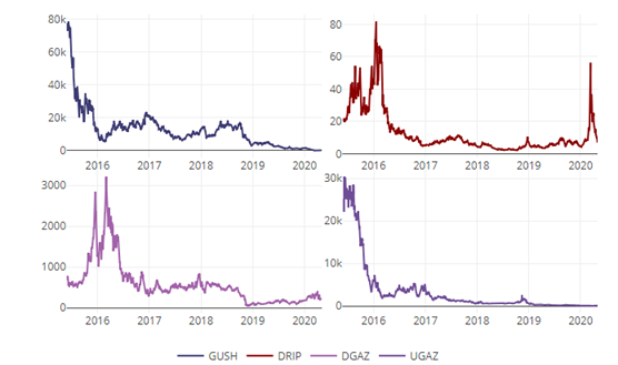
The leveraged energy ETFs examined in this paper have the distinctive feature of achieving its higher price in 2016; this is due in part to the uncertainty registered for the 2016 presidential elections in the United States and the volatility generated around energy prices. Mainly of the international oil prices from uneasiness under Trump’s policies and outcomes combined with geopolitical risks (Goldwyn, 2017). GUSH reaches its maximum value in mid-2016, breaking the 78 thousand USD. Since then, GUSH fluctuated between $20k and USD 10k. At the end of 2018, the drop in energy prices caused a sharp fall in GUSH, reaching the minimum price of $13.52. On the other hand, the DRIP price ranged between $20 to $80 from 2015 to 2016. Afterward, DRIP returned around USD 10 on average, except for the first quarter of 2020, when the price boosted to $60USD per title is shown in figure 2.
Source: Own elaboration in R programming language based on (Sievert, 2020)
a/ Data from Yahoo Finance
Figure 2 ETF’s daily closing prices from June 2015 to April 2020
In the first week of March 2020, oil prices slumped by 30% due to the conflict between Saudi Arabia and the Organization of the Petroleum Exporting Countries (OPEC); Russia and Saudi Arabia refused to implement a shortage of production proposed by OPEC (World Bank, 2020). This led to a 28.18% decrease in OPEC oil prices ($34.71 per barrel on average); the Brent crude price fell 22.52%, meaning $35.33 per barrel while West Texas Intermediate (WTI) crude price dropped to 24.52% (31.05 per barrel). DGAZ and UGAZ have similar behavior to GUSH and DRIP but with a different price range. Nevertheless, DAGZ's price did not reflect a sharp rise in the first quarter of 2020 despite the adverse oil price scenario. This effect can be attributed to the ETF structure and underlying tracking index: S&P GSCI Natural Gas Index.
Regarding volatility clustering, the most significant concentrations are the first quarter of 2020 for GUSH, presenting a negative return over 100% while DUST reaches a 50% return in one day; DGAZ and UGAZ exhibited their highest volatility at the end of 2018 with a ±50% return. According to (OPEC, 2019), the world lower demand and economic expectations in 2019 led to heavy losses for hedge fund and money managers, despite the increase of long positions on futures and options of WTI and BRET. Figure 3 represents the ETF’s volatility clustering.
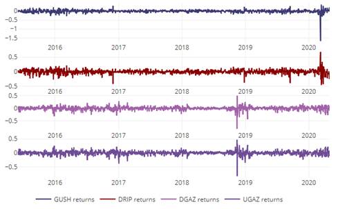
Source: Own elaboration in R programming language based on (Sievert, 2020)
Figure 3 ETF’s volatility clustering (logarithmic returns) from June 2015 to April 2020
Finally, the leptokurtosis observed in the energy ETFs is more marked in the reverse shares: DGAZ and DRIP, showing an over-cumulation of frequencies around mean and extreme tails by outliers returns (more loaded in the negative side of the distribution). Contrarily, GUSH and UGAZ display less narrow concentration, as seen in figure 4.
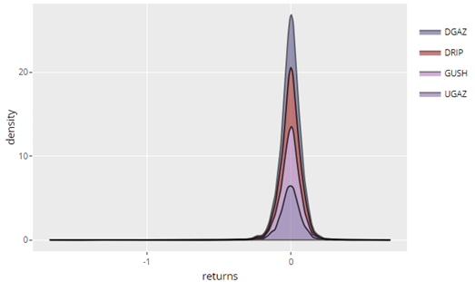
Source: Own elaboration in R programming language based on (Wickham, 2020)
Figure 4 ETF’s returns stack density
Rolling window mean-return model
When calculating the standard deviation and return of an asset or a basket of assets (investment portfolios), there is a risk of misleading episodes of high volatility, since most of the time the analysis is made from the size of the sample (considering at least one year to build investment portfolios). This section's purpose is to show the advantages of implementing rolling standard deviation or rolling volatility in shorter timeframes. This allows us to consider risk-loving profiles who can profit in daily trading.
We start from the traditional standard deviation formula. ETF's analysis is done individually, as it seeks the most profitable opportunity for each party and not jointly. Thus, the standard deviation of each of the energy leveraged ETF's is calculated:
Where σ is the standard deviation or volatility of every ETF,
Where
Table 3 Performance metrics for all sampling
| ETF | Return | Standard Deviation | Sharpe |
|---|---|---|---|
| GUSH | -155% | 1.3653 | -1.1352 |
| DRIP | -22% | 1.2210 | -0.5189 |
| DGAZ | -26% | 1.2291 | -0.5553 |
| UGAZ | -137% | 1.2170 | -0.7351 |
Source: Own elaboration
Table 3 performance metrics suggest a terrible picture for energy leveraged ETF; the bull ones, GUSH and UGAZ, presented the worst negative return (-155% and -137% individually) while DRIP and DGAZ registered -22% and -26% annualized returns respectively. Yields are so unfavorable that the Sharpe ratio implies that there is no risk compensation for the return gained. If we turn these performance metrics into a rolling window, we can know these parameters dynamically. Figure 5 represents the annualized mean and volatility performance in a rolling 252-days window.
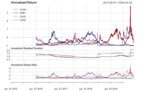
Source: Own elaboration in R programming language based on (Peterson & Carl, 2020)
Figure 5 Rolling annualized mean and volatility performance (252 days)
By categorizing daily return and standard deviation as seen in figure 5, it is confirmed that DRIP and DGAZ, the bears ETFs registered their best return performance in 2019 and February 2020 (10 to 30% return) while GUSH and UGAZ only showed a near 10% return the first quarter of 2017 and mid-2018. Standard deviation reaches its highest level for all ETFs (mainly GUSH and DRIP) in the first quarter of 2020. Recall that the Sharpe ratio suggests an appropriate risk-return relationship since 2019 for DRIP and 2020 for DGAZ.
Another approach to analyzing risk-return dynamics is by making shorter timeframes. When relating monthly performance with a rolling window of 20 days specification, a new scenario is a model; this is useful for swing and daily trading2 positions. Nevertheless, we highlight that this paper is not focused on buy and sell signals. Still, to hypothesize about a better understanding of risk-return behavior through large spikes formation and its relation to return performance in different pictures, this means different timeframes. We use the following specification for monthly rolling windows (20 days since these ETFs are not traded on weekends).
Where
Figure 6 shows the performance of rolling risk-return for GUSH and DRIP. The Rolling mean for GUSH points out an average return of ±5% except for the first quarter of 2020 had its worst performance of -20%, this same quarter, the standard deviation for GUSH soared. Diversely, both DRIP's return and volatility boosted in March 2020 as oil prices plunged.
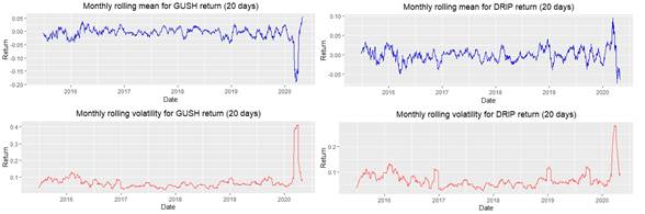
Source: Own elaboration in R programming language based on (Jeffrey & Ulrich, 2020)
Figure 6 GUSH and DRIP rolling risk-return performance (20 days)
On the other hand, DGAZ and UGAZ exhibited their highest volatility at the end of 2019, while DGAZ dropped to -8% return, and UGAZ only decreased by 0.75%. In both cases, there is an uptorn in the standard of the first quarter of 2020, representing a negative return for DGAZ and a gradual recovery for UGAZ. Figure 7 refers to DGAZ and UGAZ rolling risk-return performance.
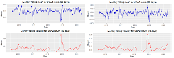
Source: Own elaboration in R programming language based on (Jeffrey & Ulrich, 2020)
Figure 7 DGAZ and UGAZ rolling risk-return performance (20 days)
To examine the relationships among the financial market and its volatility, we use the Market Beta (β), a dispersion measure of any asset compared to the overall market. Market Beta is related to S&P500 considered as one of the majors representative market index worldwide and, given the leverage of the energy ETFs used in this study, a Beta linked to β the Chicago Options Volatility Index (VIX) is estimated. Recall Beta interpretation adapted for this analysis:
Table 4 Beta coefficient interpretation
| β value | Interpretation |
|---|---|
| β > 1 | The ETF is more volatile than the overall market (S&P500) and broader market volatility (VIX) |
| β = 1 | The ETF is as volatile as the overall market (S&P500) and broader market volatility (VIX) |
| β = 0 | The ETF is uncorrelated to the overall market (S&P500) and broader market volatility (VIX) |
| 0 < β < 1 | The ETF is less volatile than the overall market (S&P500) and broader market volatility (VIX) |
| β < 0 | The ETF is negatively correlated to the overall market (S&P500) and broader market volatility (VIX) |
Source: Own elaboration
Similar to equation 3, we use a monthly rolling beta for S&P500 and VIX for each ETF. The formula implemented is:
Where
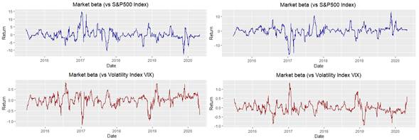
Following the description in table 4, figure 8 presents the temporary analysis of GUSH and DRIP on S&P500 and VIX. Note that in the case of GUSH vs. S&P500, it shows betas greater than zero and overall, very high arriving spends 15, in two periods, the first starting the Donald Trump administration in 2016 and a second in mid-2017. On the GUSH and VIX side, we notice negative betas, which infer an inverse relationship with the volatility index, except for a period in mid-2019, because of U.S. protectionist policy.
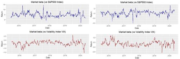
Source: Own elaboration in R programming language based on (Jeffrey & Ulrich, 2020)
Figure 8 GUSH and DRIP market beta vs. S&500 and VIX
DRIP's market beta is in most of the time series strongly negatively correlated to the overall market (S&P500) as expected according to its feature as inverse ETF just in points as the last quarterly 2016 and the first quarter of 2020 due to uncertainty perceived as previously mentioned, provoked a positive correlation with (S&P500). On the other hand, it is shown positive market volatility no bigger than one, but it turns negative in points as in the middle term of 2019 and March 2020.
Source: Own elaboration in R programming language based on (Jeffrey & Ulrich, 2020)
Figure 9 DGAZ and UGAZ market beta vs. S&500 and VIX
Regarding DGAZ in figure 9, its market beta is correlated on both sides (positive and negative) to the S&P500 index, and more volatile compared to S&P500 across the time spotted, this peculiarity makes it more complicated to fit it as an opponent even if it is an inverse ETF, the outliers returns and loses are explained by the events exposed, in the case of facing return against VIX, the market volatility is contained in values -1 and 1, then it has a broader market volatility.
We examined that the leveraged energy ETFs have a distinctive feature of achieving its higher price in uncertainty registered for the 2016 presidential elections in the United States and the volatility generated around energy prices. Then we analyzed the leptokurtosis observed in the energy ETFs. Whit the methodology proposed, we find rolling annualized mean and volatility performance. Finally, we compare the beta market with S&500 and VIX as volatility references.
5. Conclusion and Futures Works
Nowadays, ETF has become alternative financial instruments for those agents who are looking to profit in bear or bull markets, our purpose about employing rolling standard deviation in shorter time frames let us catch high volatility generated around energy prices for the sake of implementing it in an investment strategy for those risk-loving profiles that could yield broader gains from daily trading. It is important to point out that by splitting into annual and monthly timeframes, it could be implemented swing strategies by holding leveraged ETF's for a few days.
The leveraged or inverse ETFs discussed in this article allow us to make an investment choice depending on price direction expectation of the S&P GSCI Natural Gas Index (for DGAZ and UGAZ) and Oil & Gas Exploration & Production companies with GUSH and DRIP. When trading in the market, it is imperative to get knowledge about the sector we are into, as we noticed, one of the main advantages of ETFs is that they can transmit information about energy assets (in this case), subsequently average returns and market beta linked to S&P500 and VIX should be a good estimation of risk-performance exposure.
Our work's main contribution is the use of rolling volatility on leveraged ETF to understand better how this volatility has changed over time or behaved in different market conditions. Rolling deviations, viewed from different time frames (monthly and yearly in this case), allows us to hypothesize about antecedent causes and future probabilities of large spikes with the support of the rolling market beta over the Volatility Index. In that sense, our proposal allows us to dynamically rebalance investment decision making to manage volatility better from episodes of high volatility seen in rolling windows.
ETFs leveraged structure is critical because of its high risk-return expectation. In general, ETFs are a mechanism for investors to foresee the future structure of price to make decisions about an efficient allocation of resources. The ETFs split or inverse split provides a massive explanation of hasty-value changing that is a matter for future research to get what investors are waiting for, due to this process. So, in the end, which is more profitable, bull or bear ETFs? Both exhibit extraordinary profits in turn of a higher-risk compensation (maybe not worthy for an adverse risk investor). The methodology presented can make the rolling windows as small or as large as wanted, depending on the timeframe in which the investor is interested in analyzing the risk-return relationship. Nevertheless, when volatility negatively affects energy prices, bear leveraged energy ETF’s volatility, and return go nuts.

