


 nueva página del texto (beta)
 Inglés (pdf)
 Artículo en XML
 Referencias del artículo
 Enviar artículo por email
 Citado por SciELO
  Similares en
SciELO
Similares en
SciELO 
 Permalink
1. Introduction
Algorithmic trading4 is used to whether to find a top or bottom trends for shares, more specifically, investors who rely on algorithmic ttrading use quantitative and technical analysis tools to determine strategies for trade. Algorithmic trading consists of analyzing stock prices through technical charts and mathematical tools that represent open, high, low, and close prices.
Algorithmic trading seeks to detect and predict patterns in security prices; in this regard, many attempts and methodologies have been developed. This field has numerous investigations to apply techniques such as genetic algorithm (Chien-Feng, Hsu, Chi-Chung, Chang, & Chen-An, 2015), (Ying-Hua & Ming-Sheng, 2017), machine learning (Stanković, Marković, & Stojanović, 2015), (Dias-Paivaa, Nogueira-Cardoso, Peixoto-Hanaoka, & Moreira-Duarte, 2019), Bayesian models (Bian-Du & Jingdong, 2016),fuzzy time series (Gradojevic & Gençay, 2013), high frequency (Menkveld, 2013), (Hasbrouck & Saar, 2013), (Hagströmer & Nordén, 2013), technical trading rules (Bajgrowicz & Scaillet, 2012), (Kuang, Schröder, & Wang, 2014) and the development of new tools for technical analysis.
Most of the techniques mentioned apply trading algorithms that in the field of finance represents an environment where computer programs, statistical software and the developing of languages and tools, based on trading rules, are built anytime and anywhere in the world. Algorithmic trading is used for any securities since currencies, commodities, assets, or stocks. There are two types of algo-trading: 1) high-frequency trading where the trader’s advantage is in the speed of the connection and 2) low-frequency trading where the gain is in the trading model. From amateur to institutional investors who want to buy and sell such securities and get a profit (Manahov, Hudson, & Gebka, 2014).
Even though the bases of trading are quite simple -buy low and sell high- the complication is how much to buy or sell and when (Escobar, Moreno, & Múnera, 2013). Since the financial market, as a complex system, involves a high number of interacting participants to maximize profits. However, financial markets are influenced by other factors such as politics, culture, and even macroeconomics news (Lan, Zhang, & Xiong, 2011), (Escobar et al., 2013) and (Scholtus, Van Dijk, & Frijns, 2014).
Although financial markets represent a complex system, this does not mean that it is an entirely random and unpredictable system (Lan et al., 2011). Unlike the researches mentioned, it is considered that focusing on persistence and memory of patterns could lead us to build a solid strategy for trading. The motivation is not only to gain the maximum profit; the essential idea is to provide a tool that allows capturing persistence, memory, and the cyclical behavior of the financial series5. It is anticipated that prices of securities that are considered for the study could not present a random walk process since prices are hardly independent or identically distributed -at least in the financial environment-.
However, when considering a market with semi-strong efficiency where price formation is represented by the expectation of historical returns, coupled with available public information, prices can be "read" with the use of algorithms, allowing us to understand and even anticipate (at least partially) the prices and behavior without claiming that the market is efficient in the sense as is defined by the Efficient Market Theory (EMH) according to (Fama, 1969).
The basis of the algorithm for this study focuses on the use of a low-frequency model. The strategy does not depend on the speed or computing capacity of the hardware or software, in this case, the low-frequency model is formed by information retrieved from fundamentals, macroeconomic news, and financial analysts as well as strategies based on statistical and mathematical models and technical analysis which focuses on price trends and momentum (Harris & Yilmaz, 2009) and (Serban, 2010).
Under the hypothesis of whether securities show repetitive behaviors, algorithmic trading allows capturing its memory and persistence. This investigation aims to build a set of algorithmic trading strategies to capture persistence and memory of financial series. The main objectives are 1) to build an algorithmic trading strategy based on a low-frequency algorithmic trading model for daily frequency assets in a semi-strong environment and 2) to make an evaluation and optimization of the algorithmic trading strategy with a walk forward cross-validation.
HUELUM6trading System is proposed, and it is tested with (ETF) iShares NAFTRAC daily prices (ticker: NAFTRACISHRS.MX) which replicates the behavior of the Índice de Precios y Cotizaciones (IPC) in 99%, and it is the most traded ETF in México. The evaluation of the algorithm focuses on one natural calendar year from January 2nd, 2018 to December 31st, 2018: 252 observations.
Unlike other algorithms that are used to find buy and sell signals and despite of the furor of high frequency algorithms that dominate the market through their famous robot advisors and all the plentiful techniques’ applied to algorithm trading, HUELUM Trading System is built in a low-frequency environment, attending the problem of low deepness and liquidity exhibited by securities with low marketability. Likewise, HUELUM can adapt to any security as long as it has Open, High Low Close (OHLC) prices.
The document is divided as follows: the next section concentrates on the theoretical base of the study, which is the EMH Theory. The third part gives an overview of chart pattern recognition with technical analysis and Dow Theory besides the description of the tools that will be implemented. The fourth section introduces the trading System with the low-frequency model name as HUELUM. In the last part, the low-frequency trading System is optimized and tested with a walk forward cross-validation. Finally, the findings and conclusions of the study are presented.
2. Algorithmic trading on Efficiency Market Theory
Since (Fama, 1969) publication where is formally proposed the Efficient Market Hypothesis (EMH), thousands of articles have been written either to confront or provide evidence that denies/accept this hypothesis. Despite this, it has been nearly 50 years of his study and that there have been achieving in statistical, econometrics and theoretical models and even though the growing quality and quantity of financial data, as (Sewell, 2012) points out, yet and surprisingly, there is no consensus about whether a market is efficient or not.
As (Fama, 1969) defines, we can assume that a market7 is efficient if prices always “fully reflect” all available information meaning that security’s current price is equal to its fundamental value or intrinsic value. To prove efficiency, it is necessary to specify the price formation process. Using (Fama, 1969) notation:
Where E corresponds to the expected value, the price of a particular financial asset
at the time t is
Following EMH, we can distinguish among three types of market efficiency: weak, semi-strong, and strong. The first one refers to a set of information that only includes history prices; semi-strong efficiency is, in addition to history prices, the readiness of public information (e.g., annual reports, utilities, and even macroeconomics news) and the strong way means the sum of semi-strong plus private information (such as monopolistic access to relevant information about prices).
At this point, it is worth noting to highlight, which are the conditions under a market could be efficient. According to (Fama, 1969), sufficient conditions for market efficiency are:
It is assumed that there are no transactions costs8 when trading securities in the market.
Information is free and available for all market agents.
The expectative and implications of current information are thought-out and evaluated in the same way for all the market’s participants9. Hence the distributions of future security prices are known.
However, the assumptions of the theory mentioned before are restrictive, causing several criticisms and arguments against EMH. It is worth nothing to highlight some of these criticisms to explain why assuming a market in its semi-strong way allows us to approach the concept of animal spirits which includes the psychology of the traders when buying and selling securities.
2.1 Animal spirits in a semi-strong efficient market
There are plenty of publications that worn out about the failure of the EMH, but undoubtedly professor Robert Shiller is widely known for his studies that disagree with EMH theory. Part of their arguments relates to the behavior of human beings when making decisions, in other words, to what Keynes referred to as “animal spirits.”
When EMH was published in 1970, coincides with the domain of the rational expectations theory. Among the models that stood out in the financial area in 70’s -including EMH- were (Merton, 1973) whit an intertemporal general equilibrium model best known and currently widely used as Capital Asset Pricing Model (CAPM), the rational expectations general equilibrium (Lucas, 1978) which is an analysis of the stochastic behavior of equilibrium asset prices in pure exchange economy with identical consumers and one-good as well as the extension of Merton’s model published by (Breeden, 1979) where a beta of stock allows to measure the sensibility of a stock return compared to some index.
However, it was in the eighties when the boom of rational expectations started to crash down and mainly of this, at least in the financial area was because stocks began to show excess volatile behavior compared to what EMH predicted, and fundamentals changes could not explain this but for animal spirits (Shiller, 2003). In this sense, it is hardly assumed that economic agents are rational. As has been shown, in the real world, it is not possible to stand out no transactions cost and fully available information. Likewise, it is very pretentious to assume that all economic agents process the data in the same way, so we cannot expect the distributions of future securities.
Even though the criticism of EMH, if a market with semi-strong efficiency is considered as an assumption where price formation is represented by the expectation of historical returns coupled with available public information, prices can be "read" with theuse of algorithms allowing us to understand and even anticipate (at least partially) to prices behavior without claiming that the market is efficient in the sense as is defined by the EMH.
In algorithmic trading, strategy frequencies are the cornerstone before even the design of the algorithm per se, depending on the frequency of frame with which the financial asset is moving, strategies change. Frequencies for trading are: low, high, and ultrahigh (Lee & Seo, 2017).
Low-frequency trading: is done with inter day transaction regularity.
High-frequency trading: is done with intraday transaction regularity up to the minute.
Ultra-high frequency: is done with intraday transaction regularity up to the second or millisecond.
The discussion about whether a low, high or ultra-high frequency trading is the best choice to take profit in financial markets leads us to those who consider that high-frequency trading manipulates and modifies assets’ prices and market’s liquidity (Menkveld, 2013). For example, (Jacob, Napoletano, Roventini, & Fagiolo, 2016) examine the dynamic between low and high-frequency traders through an agent-based model concluding that both postures lead to flash crashes, the authors even point that high-frequency trading can be potentially harmful to financial markets stability.
Likewise, (Li, Cooper, & Vliet, 2017) point out that high frequency leads volume in financial markets but still is not clear how high frequency affect low-frequency trading. The found out that high-frequency activity improves liquidity and orderexecution quality, as well as likelihoods executions for low-frequency positions, which is a similar result from (Brogaard, et al, 2018) proving the stability of liquidity supply by high-frequency traders.
While is true that the literature of trading focuses on high-frequency and its impact on financial markets and even on low-frequency traders, these studies tend to use liquidy markets or assets, taking samples of NASDAQ or S&P500 index but what happens when there is a problem of low deepness and liquidity exhibited by securities with low marketability. The basis of the algorithm for this study focuses on the use of a low-frequency model. The strategy does not depend on the speed or computing capacity of a hardware or software; in this case, the low-frequency model is formed by:
Information retrieved from fundamentals, macroeconomic news, and financial analysts.
Strategies based on statistical and mathematical models.
Technical analysis which focuses on price trends and momentum.
It should be noted that the low-frequency model, which is proposed in Section 4, it is based on technical analysis, assuming semi-strong efficiency, transactions cost and “animal spirits” that are known as noise traders10 in EMH terms. Next section explains the nature of technicalanalysis and the mean and trend indicators that will be used for the trading System proposal.
3. Technical Analysis Chart Pattern for Securities trading
Recall the concept of noise traders or irrational traders (those who are guided by animal spirits). Empirical evidence has shown that security prices may not be as independent as they presume (Forecasts, 2015). The way that noise traders and informed traders take their decisions influence market behavior and one of the most important approaches that analyze the changes in financial markets through prices (whether an asset is bought or sold) is Dow Theory.
Dow Theory arose from a series of articles published by Charles Dow between 1900 to 1902 in The Wall Street Journal. This methodology focuses on the utilization of long term tendencies in the stock market as a measure of whether an asset goes up or down (Brown, Goetzmann, & Kumar, 1998).
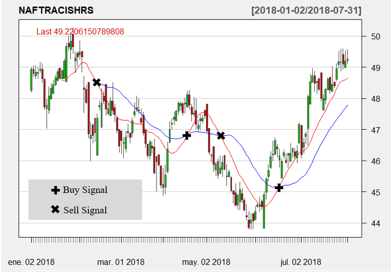
The cornerstone of the Dow Theory is that the stock market can be analyzed based on three kinds of trends: primary trend, secondary trend, and daily fluctuations. First, the prior trend is identified, although its duration and length are unpredictable, the Dow Theory and technical analysis as well make it more likely to anticipate a switch in trend. Secondary trend corrects prior tendencies; if the primary trend is bearish (downtrend), the secondary trend is called rallies. Otherwise, when the prior trendis bullish (uptrend), the secondary trend is named as corrections. Finally, daily fluctuations focus on closing averages, and they are useful for determinate long or short positions for traders. Figure 1 shows an example of a trend Theory by Charles Dow whit NAFTRAC.

Source: Own elaboration in R programming language based on “quantstrat” and “blotter” packages.
Figure 1 Dow Theory for NAFTRAC 2018-05 to 2018-12
Figure 1 shows a downtrend from June 2018 to the beginning of September 2018 but notices that there are corrections in each month of the period, after that in the middle of October a bearish trend started until December 2018 with rallies each month either. Dow Theory focuses on trend analysis of securities prices; for that reason, the use of graphs is vital to identify the market behavior that an asset follows, this is when technical analysis becomes quite useful, despite the questioning and enigma represented by this tool (Kuang et al., 2014).
Technical analysis focuses on pattern formation trough Japanese candlesticks and a universe of trading rules, which includes the use of indicators, oscillators, and even geometrical figures. Japanese candlesticks represent the open, high, low, and close (OHLC) prices of an asset. It should be noted that technical analysis is a short-term analysis and that the candlestick represents the synthesis of the prices mentioned above. As from the position of the prices, candlesticks can be bullish or bearish; high and low prices represent the tails or shadows of the body of the candle as can be seen in figure 2:

First green candle of figure 2 refers to a bull figure; this formation occurs when the close price is higher than the open price of the asset, likewise, is related to bulls because the way that they attack is with the horns (upwards). In the other hand, there is a bear figure, and this formation is done when the open price is greater than the close price and is referred to bears because these creatures attack downwards with their claws. Both bullish and bearish candles have shadows or tails; upper/lower shadows represent the distance between open/close prices and high/low prices. For this reason, it is crucial to have OHLC prices for candlesticks formation11.
From the combination of prices, different candles can be formed with both: bulls and bearers. Figure 3 shows a general classification of Japanese candlesticks that arose from the combination of those prices. The first candle (1) of figure 3 presents a biggreen body with small tails; it represents a confirmation signal of a bullish trend. The second candle (2) has the same meaning but for a downtrend. The candles numbered as 3 (short tails and bodies) suggest a hold position where neither buyers and sellers pressure the market. These candles are associated with uncertainty, and they are named as dojis12. Candles numbered 4, and 5 (long tails and small bodies) represent a trend reversal signal, both green candles are called as a hammer and inverted hammer respectively, and red candles are known as hanging man and shooting star. Finally, candles numbered as 6 (long tails and small bodies) indicate domain by buyers or sellers during the trading session. In the end, the open and close prices are relatively close, showing a sign of uncertainty in the market.

3.1 trading strategy with trend and mean indicators
The main categories for the implementation of trading strategies, at least for this proposal, are trend following and mean reversion. These strategies try to identify asset price uptrend, downtrends, and their momentum, which is the tendency of raising or falling prices to keep doing so. While is true that we can find plenty of technical indicators, for this study it will be described those that are implemented in the low-frequency algorithmic trading model proposed which are Simple Moving Average (SMA) for trend following and Bollinger Bands (BB) for mean reversion indicators.
3.1.1 Trend following indicator: Simple Moving Average (SMA)
Overall, moving averages are one of the most used and straightforward technical indicators but powerful if it is well implemented. A Simple Moving Average (SMA) is a smoothing of a time series, this case, of a security price which calculates the average of closing prices in a certain period (minutes, hours, days, weeks and so on) and is a versatile tool because SMA moves forward in time (Droke, 2001). An SMA is calculated as follow:
Where n refers to the number of observations considerate from a given period. The selection of the days for the construction of the SMA helps to capture different trend frames; as the SMA increases, the smoother the series became. According to (Droke, 2001), there are many moving averages combinations, but at the end, it is about combining fast and slow moving averages to identify crossovers, this is bull and bear signals.
Table 1 Trend frame from smoothing days for moving averages
| Trend | Moving Average |
|---|---|
| Very short term | 5-13 days |
| Short term | 14-25 days |
| Medium term | 26-49 days |
| Medium-long term | 50-100 days |
| Long term | 100-200 days |
Source: Own elaboration based on (Droke, 2001).
The way that is found a buy/sell signal is trough out the double crossover of SMA: this is when slow SMA crosses above or below a fast one. Figure 4 shows buy and sell signals trough moving averages crossovers. When the faster SMA, in this case, the 15 short average crosses below the slower SMA, this is, the 30-medium long average (the smoother), it is considered as a sell signal. Otherwise, when the faster SMA crosses above the SMA(30), then it is a buy signal. This is how SMA’s combinations become useful because, trough out its crossover, it is possible to find buy and sell signal in securities prices. However, one of the most certain challenges is to find combinations that help to detect signals in an accurately way; this is going to be possible in the Automated trading System proposed.
3.1.2 Mean reversion indicator: Bollinger Bands (BB)
John Bollinger created Bollinger Bands in 1992, and they are still widely used for technical analysts (Bollinger, 2002). It has the distinction of being based on the volatility of 20 days SMA and is an advisor for possible overbought and oversold areas13 (Bollinger, 1992). Its construction is shown as follows:
Where
Source: Own elaboration in R programming language based on “quantstrat” and “blotter” packages.
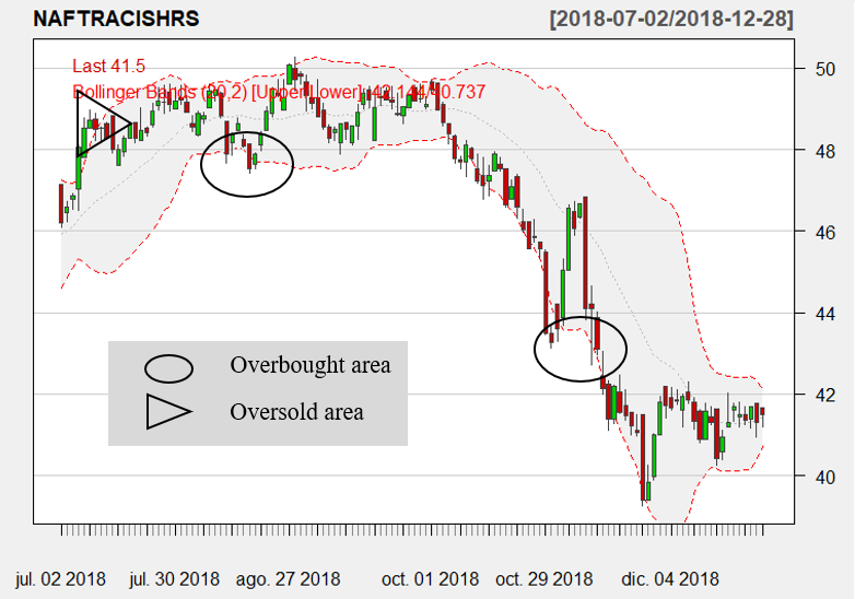
Figure 5 NAFTRAC Bollinger Bands(20,2) mean reversion strategy 2018/07 to 2018/12
In figure 5 it is observed from July 2018 to October 2018 that the NAFTRAC is in a neutral or lateral trend, the upper and lower bands are relative close each which means that there is low volatility; when BB is getting wider, these are associated to morevolatility (Bollinger, 2002). Now, when candlesticks touch upper and lower bands, for example, the two candles that are slightly up at the beginning of July 2018, these candles when arising the upper band, they bounce off, in that sense, the ETF is overbought providing a possible selling signal. In the other hand, when the closing prices or the candlestick tend to break lower bands, is consider that the security is found in an oversold area, showing buy signals14 (Bollinger, 2002).
4. HUELUM Trading System
The steps for building and testing HUELUM Trading System are:
Define the trading strategy with technical indicators.
Add strategy signals (crossover or a threshold signal).
Add enter and exit rules in market or limited positions, furthermore, stop loss, and trailing stops rules15 can be upheld.
Optimize strategy parameters using different combinations.
Evaluate the performance of HUELUM Trading System with:
Make a cross-validation process with a set training taken from sample data and tested out of the sample, in this case, a Walk Forward Analysis (WFA).
Compare strategy performance with the benchmark (buy and hold strategy).
4.1 The trading strategy, signals, and rules for HUELUM
The indicators used in this analysis are SMA (trend strategy) and BB (mean strategy). The first step is to build a double crossover trading signal; this is when indicators cross above/under between them.
Trend strategy with SMA, double crossover trading signals:
Buy signal: previous
Sell signal: previous
Mean strategy with BB, double crossover trading signals:
Buy signal: previous
Sell signal: previous
For the simulations, the following assumptions are considered:
Our initial equity is of $10,000.00 (USD).
Only market orders are allowed.
There is a transaction fee of 0.25% for each trade (buy and sell).
Every time that the buy signal is activated, 100 shares of NAFTRAC are bought.
Every time that the sell signal is activated, all the shares of NAFTRAC are sold.
NAFTRAC shares are in MXN currency. However, the results of the strategy reflect profits and losses in dollars.
HUELUM Trading System focuses on the last natural calendar year: January 2nd, 2018 to December 31st, 2018: 252 observations.
4.2 Optimization of parameters for HUELUM
Parameter optimization relies on finding a set of indicators parameters able to maximize historical risk-adjusted performance. Specifically, what is going to be done is parallel computing of sets combinations to find and chose those that report more net trading profit and loss, maximum drawdown, and profit to maximum drawdown. These combinations are going to be compared with market orders. It the end, traders will be able to choose the strategies that are more convenient to its risk profile.
In the case of the SMA strategy, its optimization will involve the calculation of the historical performance of different combinations of moving average lengths using the historical sample from January 2nd, 2018 to December 31th, 2018. So, the first part of SMA’s strategy optimization is to set different combinations of low and fast SMA.
Table 2 reports combinations of fast SMA
combinations from 10 to 20 with steps of five, and slow SMA has combinations
from 25 to 35 with the same number of steps. Results of HUELUM optimization
shows that portfolio 6 (
Table 2 Optimization of parameters for SMA Strategy
| Combinations | 1 | 2 | 3 | 4 | 5 | 6 | 7 | 8 | 9 |
|---|---|---|---|---|---|---|---|---|---|
| Fast SMA | 10 | 15 | 20 | 10 | 15 | 20 | 10 | 15 | 20 |
| Slow SMA | 25 | 25 | 25 | 30 | 30 | 30 | 35 | 35 | 35 |
| Portfolio | Port_1.1 | Port_1.2 | Port_1.3 | Port_1.4 | Port_1.5 | Port_1.6 | Port_1.7 | Port_1.8 | Port_1.9 |
| Num Txns | 9 | 9 | 13 | 8 | 10 | 8 | 8 | 8 | 6 |
| Num Trades | 4 | 4 | 6 | 4 | 5 | 4 | 4 | 4 | 3 |
| Net trading.PL | -$218.54 | -$9.58 | -$105.97 | -$354.57 | -$2.41 | $133.95 | -$224.93 | -$76.51 | -$222.16 |
| Avg Trade PL | -$54.63 | -$2.24 | -$17.66 | -$88.64 | -$0.48 | $33.49 | -$56.23 | -$19.13 | -$74.05 |
| Max. Drawdown | -$328.29 | -$199.50 | -$283.31 | -$423.95 | -$201.26 | -$200.95 | -$316.95 | -$296.36 | -$364.17 |
| Profit. To Max. Draw | -$0.67 | -$0.05 | -$0.37 | -$0.84 | -$0.01 | $0.67 | -$0.71 | -$0.26 | -$0.61 |
| End Equity | -$218.54 | -$9.58 | -$105.97 | -$354.57 | -$2.41 | $133.95 | -$224.93 | -$76.51 | -$222.16 |
Source: Own elaboration
Results are validated with figure 6; the most significant way to determine the best optimization parameters is choosing the lines that are at the top of each frame in figure 6.

Source: Own elaboration in R programming language based on “quantstrat” and “blotter” packages.
Figure 6 Strategy optimization of SMA with net trading, maximum drawdown, and profit to maximum Drawdown
The same dynamic is going to be for parameter optimization for BB strategy; table 3 reports SMA combinations from 5 to
15 with steps of five and two to three standard deviations each. In this case,
results of HUELUM optimization shows that the first portfolio (
Table 3 Optimization of parameters for BB strategy
| Combinations | 1 | 2 | 3 | 4 | 5 | 6 |
|---|---|---|---|---|---|---|
| SMA | 5 | 10 | 15 | 5 | 10 | 15 |
| Standard deviation | 2 | 2 | 2 | 3 | 3 | 3 |
| Portfolio | Port 2.1 | Port 2.2 | Port 2.3 | Port 2.4 | Port 2.5 | Port 2.6 |
| Num Txns | 36 | 20 | 13 | 8 | 3 | 5 |
| Num Trades | 10 | 3 | 1 | 4 | 1 | 1 |
| Net trading.PL | $638.11 | -$2,092.59 | -$3,193.71 | $162.60 | $45.62 | -$880.13 |
| Avg Trade PL | $63.81 | $79.75 | -$48.17 | $40.65 | -$10.64 | -$84.61 |
| Max. Drawdown | -$1,645.04 | -$3,724.33 | -$5,305.55 | -$428.29 | -$233.71 | -$1,451.94 |
| Profit. To Max. Draw | $0.39 | -$0.56 | -$0.60 | $0.38 | $0.20 | -$0.61 |
| End Equity | $638.11 | -$2,092.59 | -$3,193.71 | $162.60 | $45.62 | -$880.13 |
Source: Own elaboration
Strategy optimization is confirmed in figure 7, recall the best optimization parameters is choosing the lines that are at the top of each frame.

4.3 Rolling walk forward analysis
The cross-validation process that is going to be used for HUELUM Trading System is a Walk Forward Analysis (WFA) which consists in optimizing indicator parameters with a set training taken from sample data and is tested out of the sample repeating the process of one step forward up to the end of data time series. According to (Pardo, 2008) the main advantage of using WFA is that optimize parameters over time, in that sense, every time that the parameters are tested out of the sample, are not the same. Figure 8 represents the essence of a WFA:
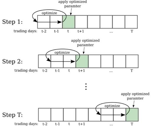
WFA allows to solve overfitting problems and is considered as a more practical method for real-time data since every time that new data is registered, is adapting to market changes. Another advantage is that is possible to know if the last optimal parameters are good enough for implement a trading strategy, if performance is not satisfactory, is likely to change to another technical indicator or to set up different parameters to be optimized. For SMA and BB indicators proposed in this work, the WFA is going to be tested with the best parameters optimization.
According to (Pardo, 2008), the size of the walk-forward window is based on data availability and data frequency. The longer the training periods, the higher the number of walk-forward, and the reliability of the WFA. Besides, a walk-forward window is proportional to the size of the optimization window. In this case, the optimal window is two months (considering slow SMA, which implies a little more than a month) and uses 10 months of training periods to perform a robust WFA. Table 4 shows the components of WFA.
Table 4 Out of sample/testing range strategy
| Training periods | 10 months |
| Testing (out of the sample) | 2 months |
| Parameters Combinations | |
| SMA Trend Strategy | |
| Fast SMA | 20 |
| Slow SMA | 35 |
| BB Mean Strategy | |
| SMA | 5 |
| Standard Deviation | 2 |
Source: own elaboration
For SMA strategy, the first testing out of the sample is from 26/04/2018 to 16/05/2018 where the de net trading is -$181.29, while is true that the net trading is not a positive amount, the optimal in this case is to minimize losses (same situation 09/10/2018 to 15/10/2018). In the other hand, WFA from 22/06/2018 to 29/08/2018 and 11/09/2018 to 27/09/2018 shows a profit of $345.86 and $54.81 respectively: results out of the sample for SMA are in table 5.
Table 5 Strategy Walk Forward Analysis Results for
| Out of Sample WFA | Trades | Net trading PL |
|---|---|---|
| 26/04/2018 to 16/05/2018 | 2 | -$181.29 |
| 22/06/2018 to 29/08/2018 | 2 | $345.86 |
| 11/09/2018 to 27/09/2018 | 2 | $54.81 |
| 09/10/2018 to 15/10/2018 | 2 | -$85.44 |
Source: own elaboration
Finally,
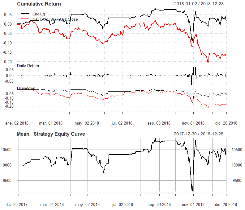
Source: Own elaboration in R programming language based on “quantstrat” and “blotter” packages
Figure 9
For
Table 6 Strategy Walk Forward Analysis Results for
| Out of Sample WFA | Trades | Net trading PL | Out of Sample WFA | Trades | Net trading PL |
|---|---|---|---|---|---|
| 24/01/2018 to 24/01/2018 | 2 | -$11.93 | 02/08/2018 to 08/08/2018 | 2 | $65.80 |
| 09/02/2018 to 09/03/2018 | 4 | $82.91 | 13/08/2018 to 28/08/2018 | 3 | $268.64 |
| 16/03/2018 to 05/04/2018 | 4 | $267.71 | 04/09/2018 to 12/09/2018 | 2 | $11.39 |
| 25/04/2018 to 08/06/2018 | 5 | -$182.32 | 03/10/2018 to 06/11/2018 | 6 | -$288.61 |
| 16/07/2018 to 25/07/2018 | 2 | $93.53 | 09/11/2018 to27/12/2018 | 5 | -$138.65 |
Source: own elaboration
In the same way as
Source: Own elaboration in R programming language based on “quantstrat” and “blotter” packages
Figure 10
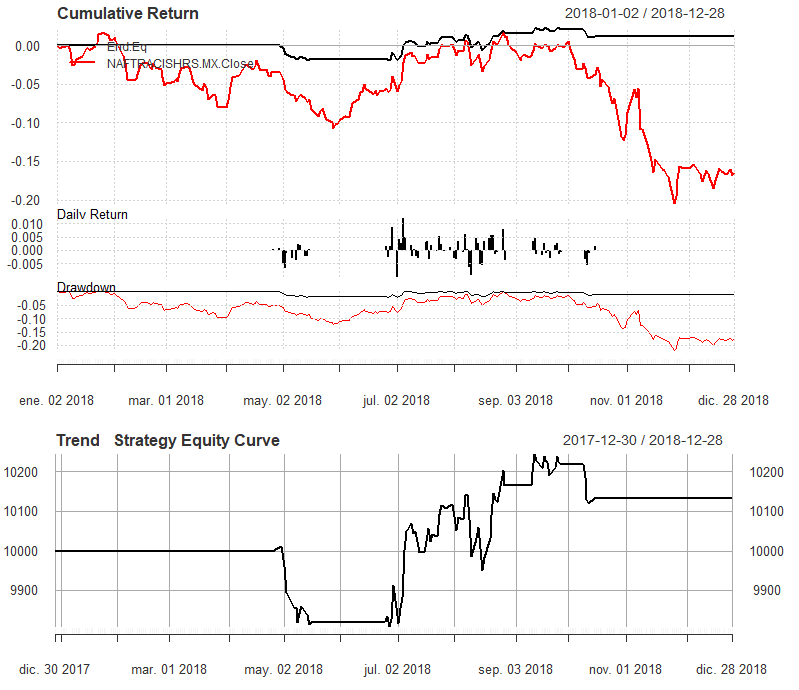
Lastly, both strategies display better trading performance
metrics compared with the buy and hold strategy.
Table 7 trading performance metrics
| Performance | SMA Strategy | BB strategy | NAFTRAC Closing Price |
|---|---|---|---|
| Annualized Return | 1.31% | 1.93% | -16.73% |
| Annualized Std Dev | 3.44% | 17.40% | 16.65% |
Source: own elaboration
While NAFTRAC ended up with a negative return in 2018, HUELUM can take advantage of NAFTRAC behavior optimizing the strategies presenting a profit.
5. Conclusions
Algorithmic trading is used to whether to find a top or bottom trends for share prices, more specifically, investors who rely on algorithmic trading use quantitative and technical analysis tools to determine strategies for trade. Algorithmic trading consists of analyzing stock prices through charts and mathematical tools that represent open, high, low, and close prices. In this regard, the objective of this work is to build a set of algorithmic trading strategies to capture persistence and memory of financial series, more specifically, to build an algorithmic trading strategy based on a low-frequency algorithmic trading model for daily frequency assets in a semi-strong environment.
HUELUM Trading System low-frequency model was proposed to make algorithmic trading tested with the ETF NAFTRAC daily prices which replicate the behavior of the Índice de Precios y Cotizaciones (IPC) of Mexican Stock Exchange. In this first version of HUELUM it was tested one mean indicator (Bollinger Bands), and one trend indicator (SMA) and they were compared to a benchmark, in this case, with a buy & hold strategy. Assuming initial equity of $10,000.00 (USD), technical indicators were probed to detect buying and selling signals: both, SMA and BB were tested applying different combinations and validated through a rolling walk forward analysis.
To select the best portfolio with SMA and BB combinations, we searched for parameters able to maximize historical risk-adjusted performance such as net trading, profit and loss, maximum drawdown, and profit to maximum drawdown. In the end, the best combinations were those its end equity exhibited the highest profit. Likewise, it is possible to know the number of trades and transactions of each combination as well as the average profit/loss per trade.
For NAFTRAC, the best technical indicators are
In the end, these strategies help to reach out the maximum profit even when NAFTRAC ended up with -16.73% annualized return. The cross-validation process implemented was a WFA which consists in optimizing indicator parameters with a set training (10 months in this case) and two months tested out of the sample repeating the process of one step forward up to the end of NAFTRAC series. WFA allows to solve overfitting problems and shows the net trading profit/loss for each out of sample and trades. WFA provides essential information about the strategy performance for each window tested.
In that sense, HUELUM could be used for a general strategy or could be tested in every time frame chosen from the trader to select the most profitable indicator or a mix of technical indicators which is a notable advantage since is possible to track trades and strategy performance through an equity curve graph whether form general strategy or WFA windows.
The main of this work is that the HUELUM Trading System has the capability to adapt to any asset (as long as it has OHLC prices), to capture its behavior, trends and momentum and even better, HUELUM gives accurate buy and sell signals allowing trading strategies, all of this, in a low-frequency environment. It is worth noting to point out that while it is true that this research only reported market positions, HUELUM has the flexibility to include limited, stop loss and trailing stops positions according to trader’s preference. Recall the possibility to change cost transactions in HUELUM, which allows comparing different fees, another advantage of this trading System.
Although high-frequency algorithms have become the sensation for many analysts and traders, keep in mind that not all the markets have the deepness and liquidity to make that high-frequency algorithm works efficiently, especially securities that are listed in emerging countries such like México. This is when algorithm trading for low frequency like HUELUM, helps to traders, to analyst and anyone who has an investment in financial assets, to make a better an accurate decision compared to a buy &hold strategy, to make more profits and last but not least, to reduce potential equity losses.
Now, this is not the first and last version of HUELUM; this trading System has the flexibility to include other indicators, not necessarily technical ones. For future research, the creation of new tools and indicators will be implemented in HUELUM Trading System.

