


 nueva página del texto (beta)
 Inglés (pdf)
 Artículo en XML
 Referencias del artículo
 Enviar artículo por email
 Citado por SciELO
  Similares en
SciELO
Similares en
SciELO 
 Permalink
1. Introduction
There is a robust body of literature that explains the benefits of Microfinance Institutions (MFIs) for low-income people, highlighting improvements in their income and well-being.2 However, since their creation, MFIs have served those with a low-income and at the same time sought financial self-sufficiency. Regarding self-sufficiency, some MFIs have applied restrictive credit policies, which are detrimental to the segment they are supposed to serve. Also, MFIs began to focus primarily on profitability at the expense of helping the poor and lowering the incidence of poverty, which is referred to as MFIs Mission Drift (MD). There exists evidence that MFIs profitability may be higher than that of commercial banks (González and Rosenberg, 2006).
In regards to MD, there are at least two perspectives in the literature. The first one analyzes the relationship between profitability and variables that measure MFI coverage of low-income people, also known as outreach (González y Rosenberg, 2006; Cull, DemirgücKunt y Morduch, 2007; Cotler and Rodríguez-Oreggia, 2008 and 2013; Alinsunurin, 2014 and, Pop, 2015, among others). Some of these studies have found weak evidence of MD, while others have found substantial evidence regarding this issue. The second perspective includes studies that address those factors related to profitability and outreach (Cull, Demirgüç-Kunt, and Morduch, 2009, 2011 and 2014; Bogan, 2012; Kar, 2012; Nwachukwu, 2014; and Pati, 2014 and 2015). The previously mentioned studies suggest how to improve these two indicators, in regards to the original MFI mission sense. For example, at a country level, studies argue that regulation damages profit and outreach; meanwhile, a developed financial system has a positive effect on outreach. At MFI level, it was found that a higher debt to equity ratio improves the financial performance.
However, as we explain in the following section, to our knowledge there is no consensus about whether or not MFI mission drift exists. Furthermore, there is no consensus about what the relevant variables concerning profitability and outreach are. In this regard, this paper aims to contribute to this debate concerning MFIs. In particular, we analyze whether a mediator variable that has a significant effect on financial performance or outreach exists. We test whether capital structure, environment (corruption, the rule of law and government inefficiency), operating efficiency, and size of the MFI have a direct or indirect effect, if any, on outreach and financial performance. This paper contributes to the MFI literature in two ways: 1) the use of Structural Equation Modeling (SEM), which allows for the analysis of indirect effects, corrects for measurement of reciprocal effects, controls for measurement errors, and allows multicollinearity. More details on the advantages of this methodology are presented in the third section: 2) the construction of the dependent and independent variables, using more than one variable from MFI literature. In the following section, the literature addressing MFI mission drift and outlining the explanatory variables of financial performance and outreach is discussed. The third section presents the structural equation modelling, data to perform the analysis as well as our results.
2. Literature review
Although the primary concern of this work is related to the variables that explain MFIs financial performance and outreach, it is essential to recognize that the source of this concern is the evidence of a relationship between these variables and the MFI mission drift. Thus, in the first part of this section, we review the literature examining mission drift through analyzing profitability and outreach, and in the second one, we review the literature concerning these two specific variables.
It is important to note that profitability is generally measured through financial self-sufficiency (FSS), which according to MIX Market is the ability of an MFI to cover its operating costs, an MFI is considered to be financially self-sustainable if the ratio of revenues over expenses is higher than 1.10. This indicator, proposed by MIX, is widely used in the microfinance literature. Other studies rely on return on equity (ROE) and return on assets (ROA) (Gutiérrez-Goiria and Unceta, 2015) as alternative variables measuring profitability. Besides, outreach includes all social impact measures, which generate a benefit to the poorest or foster women empowerment (Gutiérrez, 2012). Outreach essentially refers to the level of MFI market coverage or to the number of low-income people they serve. Although many authors have studied MFI outreach, there is no standard measure; instead it is measured by social performance variables, such as the number of clients served (range of outreach), the average size of the loan (depth of outreach), or the percentage of women borrowers (empowerment) (Vanroose and DEspallier, 2013).
2.1 MFI mission drift: profitability and outreach
In 2000, Morduch argued that higher interest rates do not necessarily imply a reduction in credit allocation. He found evidence that financial sustainability allows MFIs to have a more extensive range. Like Woller, Dunford, and Woodworth (1999), Morduch discussed the debate between institutionists and welfarists, as an example of mission drift. He found that while the objective of the former group was to increase financial sustainability and develop the credit portfolio, the objective of the latter was to eliminate extreme poverty.
In 2006, González and Rosenberg found results that reinforced the arguments for MFI mission drift; they found that 44% of MFIs are more profitable than commercial banks. Likewise, they analyze the relationship between MFI profitability and outreach, which led to evidence of mission drift. It was identified that either MFIs are profitable or wideranging, but not both. Cull et al. (2007) similarly found a weak relationship between profitability and outreach. They found that, even when an MFI is granting small loans, it does not lose profitability. They also found statistical evidence of a relationship between the size of the loan and operating cost. Their findings suggest that the higher the loan, the lower the average operating cost, which is evidence of incentives to mission drift.
Other studies, such as Cotler and Rodríguez-Oreggia (2008), have identified evidence of a significant relationship between profitability and outreach. Through a positive correlation between profitability and average loan size in a Mexican MFI sample. In their study, they suggest two alternatives to resolve the MFI mission drift concern: an increase in productivity, or a reduction in funding costs. Regarding this matter, Alinsunurin (2014) found that MFIs have not yet been able to integrate the dual objectives of profitability and social impact. Alinsunurin also found that non-profit MFIs were more efficient in social impact but less profitable than for-profit MFIs. This result is similar to that of Pop and Buys (2015), which also identified MD in Romanian MFIs. Furthermore, Pop and Buys also found that MFIs are concentrated in developed cities rather than in communities. In regards to the studies that do not support MFI mission drift, Kar (2013) found no evidence that for-profit organizations have dropped their primary objective. However, he does report an existent lack of reliable information in his study.
2.2 Explanatory variables of MFI financial performance and outreach
The literature addressing variables affecting profitability and outreach found that the legal status of MFIs has a significant impact, Cull et al. (2009). As for-profit banks grant more substantial individual loans, in proportion of total portfolio, than non-profit institutions. They also argue that non-governmental organizations have higher operating costs and lower profitability levels compared to for-profit counterparts. In 2011, the same authors established that when for-profit MFIs are regulated, they show significant profitability margins. It was also found that regulation is negatively related to outreach.
Regarding the effect of capital structure, Bogan (2012) found that the amount of equity, measured as a proportion of total assets, is relevant for both profitability and outreach. He also found that donations jeopardize sustainability by reducing operating efficiency. Like Kar (2012), he found that the higher the debt to equity ratio (leverage), the better the financial performance. However, he did not find that leverage had a significant effect on outreach. In regards to this, Pati (2014) found that because MFIs have access to a variety of financial sources, their capital structure has a significant effect on profitability.
When searching for variables that stimulate the core mission of MFIs, Cull et al. (2014) found that the more developed the financial system, measured as bank penetration through branches and ATMs per square kilometer, the higher the impact that MFIs would have on outreach to the low-income population, and in turn this is reflected in an increase of microcredits, including those for women. Pati (2015) found that capital structure, operating expenses, and asset quality are the primary drivers of MFI financial performance and outreach. When analyzing the impact of interest rates on sustainability, Nwachukwu (2014) identified an inverse U-shaped relationship between these two variables, which suggests that there is an optimal MFI interest rate. Also, she did not find any substantial evidence suggesting that small loans imply a higher sustainability risk. Balammal et al. (2016) found that legal status, the regulatory environment, the age of the MFI, number of employees, capital structure, and cost per client have a significant impact on MFI financial performance.
As discussed, in the previous studies we acknowledge a lack of consensus regarding the existence of mission drift. However, none of these studies analyzes an indirect relationship between the variables. In this work, we do not attempt to prove the existence of mission drift. Instead, we attempt to explain how specific independent variables, most commonly cited in MFI literature, affect profitability and outreach.
3. Data and methodology
We rely on information from the Mix Market Intelligence database 2015. Our study is based on a sample of 545 MFIs, which voluntarily reported their information. It is important to mention that only MFIs with complete information were selected according to methodological requirements. Table 1 conveys the distribution of MFIs by region, profit and legal status, size, and age:3
Table 1 Sample distribution according to various indicators
| By region | Profit or non-profit | By age | By legal status | By size | |||||
|---|---|---|---|---|---|---|---|---|---|
| # IMF | # IMF | # IMF | # IMF | # IMF | |||||
| Eastern Europe and Central Asia | 70 | For-profit | 264 | New: 1-4 years | 21 | Non-Bank Financial Institution | 223 | Small | 103 |
| South Asia | 123 | Non-profit | 281 | Young: 5-8 years | 71 | Credit Union / Cooperative | 68 | Medium | 111 |
| Africa | 70 | Mature: >8 years | 435 | NGO | 161 | Large | 331 | ||
| Latin America and the Caribbean | 179 | Non-specified | 18 | Bank | 65 | ||||
| East Asia and the Pacific | 89 | Other | 15 | ||||||
| The Middle East and North Africa | 14 | Rural bank | 8 | ||||||
| Non-specified | 5 | ||||||||
Source: author with data from Mix Market
An essential feature of the sample is that there exists a balance between for-profit and non-profit MFIs. Also, more than 70% of the sampled MFIs are over eight years old.
As previously mentioned, the purpose of this paper is to analyze the factors that have a direct or indirect effect on the financial performance and outreach of MFIs using Structural Equation Modeling (SEM). The use of SEM to examine strategic management phenomena has increased dramatically in the last decades (Shook, Ketchen, Hult, and Kacmar, 2004). An advantage of SEM over multiple regression analysis such as ordinary least squares (OLS), is that it can avoid potential multicollinearity when all correlated variables are simultaneously included (Qingfeng Wang, Xu Sun, 2017). In addition, the fact that SEM facilitates the analysis of a complex set of simultaneous linear relationships among multiple variables is an advantage over other techniques (Iglesias, and Lévy, 2010). On the other hand, while OLS multiple regression analysis is mainly utilized to confirm a previously established theory, covariance-based SEM models are primarily used to confirm or reject theories by determining how well a proposed theoretical model can estimate the covariance matrix of the dataset. SEM allows for the incorporation of unobservable variables that have been measured indirectly by indicator variables (Hair, Hult, Ringle and Sarstedt, 2017).
Regarding the use of SEM in the finance literature, several studies point out the advantage of SEM over multiple regression analysis. For example, Iglesias and Lévy (2010) argue that one advantage is related to a commonly adopted hypothesis found in the finance literature, this being that the idiosyncratic components of asset returns have zero correlations across assets. In regards to this, there is evidence that suggests a poor performance in models that analyze macroeconomic variables with finance variables such as asset returns because of the error measurement (Chan, Karceski and Lakonishok, 1998). SEM solves this problem by allowing the analyst to work with unobservable risk factors that are derived from a series of observable variables and an error term (Iglesias and Lévy, 2010).
Next we proceed to describe how to apply SEM methodology. SEM involves the evaluation of the measurement model and the path model. These two models are classified as confirmatory factor analysis, estimating several simultaneous equations to prove if and, eventually, how independent variables relate to the dependent variable (Lei and Wu, 2007).
A prerequisite of the SEM models is that they require large samples. According to Suhr (2006), the number of observations must be at least five times the number of variables, and must never be less than one hundred. Because we used ten independent variables and three dependent variables, our 545 observations in the sample fit this requirement. Table 2 presents the variables we used in our analysis:
Table 2 Definitions of variables
| Variable | Short name | Definition |
|---|---|---|
| Return on assets | ROA |
|
| Return on equity | ROE |
|
| Financial sustainability | OSS |
|
| Government effectiveness | KKM3 | An indicator published by The World Bank related to the perception of the population about the quality of public services and central public institutions and which also covers the credibility of policymakers.4 |
| The rule of law | KKM5 | An indicator published by The World Bank about social norms, their applicability, and the general justice system. It also covers perceptions about levels of violence and criminality. |
| Control of corruption | KKM6 | Indicator published by The World Bank about perceptions of corruption in public and private spheres. |
| Interest expense | COST_FUNDING | Expenses incurred by MFIs as part of servicing debts. |
| Equity | EQUITY | The equity book value of the MFI |
| Staff employed | LogPERSONNEL | Number of total MFI employees. |
| Active borrowers | LogACTIVEBORR | Number of people that have received at least one credit from an MFI. |
| Administrative expenses | ADMEXP_PORT | Administrative expenses as a proportion of total credit portfolio |
| Operating expenses | OPEXP_PORT | Operating expenses as a proportion of total credit portfolio |
| Personal expenses | PERSEXP_PORT | Personnel expenses as a proportion of total credit portfolio |
Source: author with data from Mix Market
In the social sciences, it is typical to use alternative measures to explain variables that cannot be observed; in econometric analysis, they are referred to as proxy variables. For example, outreach is the capacity of the MFI to reach the low-income segment, which can be approximated with the average loan size, while return on equity can represent a measure of profitability. In SEM, these variables cannot be analyzed directly. Instead, SEM attempts to incorporate unobservable variables measured indirectly by indicator variables, which facilitate measurement error to be detected in observable variables (Chin, 1998). In other words, analyzing a complex phenomenon with a single proxy variable may not be representative of it; instead, SEM creates a linear combination of several variables, referred to as latent variables or constructs, which reduce measurement error (Hair et al., 2017).
To build the constructs, we use the methodology proposed by Jarvis, Mackenzie, and Podsakoff (2003), by establishing the three following conditions: i) the indicators must characterize the constructed measure; ii) the variables of each construct must be consistent with the variable they are required to approximate (we use the Cronbach alpha to verify the concordance of each construct), and; iii) the covariance between variables and constructs must be significant (Aldás-Manzano, Lassala-Navarré, Ruíz-Mafé, y Sanz-Blas, 2011).
3.1 Effect of the environment, capital structure, operating efficiency and size on profitability.
In this section, the variables we utilize, allow us to create a construct of profitability, environment, capital structure, size and operating efficiency.
First, to measure profitability we build a construct, essentially a linear combination from ROA, ROE and OSS based on the works of Cull, Demirgüç-Kunt and Morduch (2009), Pati (2015) and Gutiérrez-Goiria and Unceta (2015); those studies intend to prove that MFIs have conflicting objectives because they do not represent a sustainable business model. The first independent variable is the Environment because according to Cull et al. (2014), the setting in which the MFIs operate is an essential determinant of both performance and outreach. For this work, based on Kauffmann et al. (2007), we built the construct with corruption control, the rule of law, and government effectiveness. Our second independent variable is the Capital Structure. For this construct, we use equity and interests’ expenses, following Pati (2014), who made a comparative study about capital structures for MFIs around the world. The third dependent variable is the Size of the MFIs. Following the studies of Cotler and Rodríguez-Oreggia (2008) and Cull et al. (2011), for this construct, we use the staff currently employed and the number of active borrowers. Finally, we formed Operation Efficiency construct, as a measure of the operating expenses.
Before proceeding to the analysis, it is necessary to examine whether the constructs meet the previously mentioned criteria from Jarvis et al. (2003) beginning with the exploratory factor analysis. In this sense, according to Nunnally (1978), this criterion is met when the Cronbach alpha is higher than 0.8, which is the case for the entire construct, as shown in Table 3. The next step is to verify the relationship among indicators through the Kaiser-Meyer-Olin (KMO) test and the Bartlett Sphericity Test. The KMO is a reliability test, which measures whether the constructs have a common variance that must be higher than 0.5. In this case, our results in Table 3 show that, except for operating efficiency, all constructs have a common variance. Also, in Table 3 we demonstrate that the Bartlett sphericity test, which measures whether the factorial construction is appropriate, is indeed significant, and the total percentage of accumulated variance as well as the contribution of each factor to it.
Table 3 Cronbach alphas and exploratory factor analysis model, financial performance model
| Items | Financial performance | Environment | Capital structure | Size | Operating efficiency |
|---|---|---|---|---|---|
| ROA | 0.944 | ||||
| OSS | 0.897 | ||||
| ROE | 0.882 | ||||
| KKM5 | 0.946 | ||||
| KKM6 | 0.893 | ||||
| KKM3 | 0.891 | ||||
| EQUITY | 0.964 | ||||
| COST_FUNDING | 0.964 | ||||
| LogPERSONNEL | 0.977 | ||||
| LogACTIVEBORR | 0.977 | ||||
| OPEXP_PORT | 0.994 | ||||
| PERSEXP_PORT | 0.928 | ||||
| ADMEXP_PORT | 0.902 | ||||
| Cronbach alpha | 0.739 | 0.89 | 0.705 | 0.949 | 0.885 |
| KMO | 0.704 | 0.703 | 0.5 | 0.5 | 0.476 |
| Bartlett chi square | 1029.919*** | 1058.583*** | 718.542*** | 951.178*** | 2371.754*** |
| % explained variance | 82.43% | 82.90% | 92.84% | 95.46% | 88.77% |
| FULL MODEL KMO | 0.626 | ||||
| Bartlett chi-square | 6742.348*** | ||||
| % of explained accumulated variance | 88.31% | ||||
| Contribution of each factor to the total variance | 19.20% | 19.22% | 14.40% | 14.81% | 20.69% |
*** p <0.01
Note: the values of the factorial loads are shown in the cursive script
Source: author
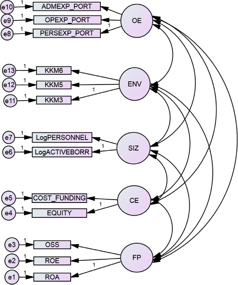
The principal component analysis is performed though the Varimax Rotation Method, which is suggested in samples that contain just a few variables in each factor, allowing maintaining a significant proportion of variance in each construct (Abdi, 2003). To evaluate the model, we use a confirmatory factor analysis (CFA). In Appendix three can be seen that for each construct, the correlation is higher than 0.8 and the variance percentage that each factor captures is higher than 80%. This result indicates that each factor is a good representative of its respective variable. In addition, it conveys statistical evidence of multicollinearity among each construct. As we previously mentioned, allowing this assumption in the model is an advantage of SE models, concerning OLS multiple regression analysis. Figure 1 shows the results of the confirmatory factor analysis.
To prove goodness-of-fit in the model, we must use more than one indicator (Feinian, Curran and Bollen, 2008). The first two parameters are the Chi-Square and chi square over degrees of freedom. In Table 5, we show that the chi-square is significant. According to Hu y Bentler (1995), whether the result of the division of the chi-square divided by the degrees of freedom is higher than two, it this implies statistical evidence that the SEM is not valid. However, Lei and Wu (2007) prove that SEM is well specified and valid if the model meets the following conditions: the sample is large enough and NFI, CFI, and GFI are over 0.9 (Bentler y Bonett, 1980; Bentler, 1989; Joreskog and Sorborn, 1986). As we can see in Table 5, there is evidence of model goodness-of-fit in our proposed model. The final goodness-of-fit is the RMSEA, which must be under 0.8, which is the case in our model (Steiger and Lind, 1980).
Table 4 The goodness of fit for financial performance
| Items | AVE | CR |
|---|---|---|
| Financial performance | 0.746 | 0.898 |
| Capital structure | 0.858 | 0.923 |
| Size | 0.931 | 0.964 |
| Environment | 0.753 | 0.901 |
| Operating efficiency | 0.861 | 0.948 |
| Chi square (CMIN) | 374.382*** | |
| CMIN / DF | 6.807 | |
| CFI | 0.953 | |
| GFI | 0.912 | |
| NFI | 0.945 | |
| RMSEA | 0.103 |
*** p <0.01
Source: author
Table 5 Discriminant validity
| FP | CE | SIZ | OE | ENV | |
|---|---|---|---|---|---|
| Financial performance (FP) | 0.746 | ||||
| Capital structure (CE) | 0.004 | 0.858 | |||
| Size (SIZ) | 0.002 | 0.275 | 0.931 | ||
| Environment (ENV) | 0.044 | 0.011 | 0 | 0.753 | |
| Operating efficiency (OE) | 0.005 | 0.001 | 0.013 | 0.003 | 0.861 |
Source: author
Following the work of Orozco-Gómez (2016), we apply a convergent and discriminant validity of SEM methodology. First, we extract the average variance (AVE) of each element of the construct. According to Carr (2002) and Fornell and Larcker (1981), this average must be over 0.5. In Table 5, we demonstrate the results of this test. As we can see, our model shows convergent validity. Additionally, we estimate the square of the correlations of each pair of factors and then compare it with the average variance extracted from each factor (Campbell and Fiske, 1959). To prove discriminant validity, the square of correlations must be less than each AVE. In Table 6, we show the AVE in the diagonal and under the respective square correlations. As we see in Table 6, our model meets the discriminant validity criteria
Table 6 Structural model estimators, financial performance
| OE | FP | |
|---|---|---|
| Operating efficiency (OE) | -0.196 (.000)*** | |
| Capital structure (CE) | -0.158 | 0.073 |
| (0.000)*** | (0.178)NS | |
| Size (Siz) | 0.089 | -0.049 |
| (0.009) *** | (0.332)NS | |
| Environment (ENV) | -0.055 | 0.059 |
| (0.059) ** | (0.176)NS |
NS: not significant, **: significance at 95%, *** 99%
Correlation between CE and SIZ = 0.566
Source: author
In this section, we analyze financial performance as a dependent variable, while we treat the other variables as an independent. We also establish a causality relationship and a maximum verisimilitude criterion. In Figure 2, we show evidence that capital structure, size, and environment do not have a significant direct effect on financial performance. Instead, the effect is through operating expense.

In Table 6, as is expected, the coefficient of the relationship between operating efficiency and financial performance is negative. The capital structure and environment coefficients are negative and significant but only for operating efficiency, not for financial performance. The same is valid for size, but with a positive sign. The latter is statistical evidence that capital structure, size, and environment do not have a significant direct effect on financial performance. Instead, the effect is through operating expense. We also tested the model without the environment measure, although the results, concerning significance, coefficients are very similar to those presented in Table 6. Our significant negative relationship between financial performance and operating efficiency result is consistent with the results of Cull, Demirgüç-Kunt and Morduch (2011 and 2014), Nwachukwu (2014) and Pati (2015). However, our result differs from the findings of Bogan (2012) and Kar (2012), as it demonstrates an indirect relationship between capital structure and financial performance through operating efficiency, as opposed to their result, which shows a direct link between these variables.
Regarding size, our result is consistent with the works of Cull et al., (2011), Bogan (2012), Pati (2014 and 2015), Kar (2012) and Gutiérrez-Goiria and Unceta (2015), Cull, Demirgüç-Kunt, and Morduch (2011 y 2014), who find a positive but not significant relationship between size and financial performance. However, unlike our case, they did not relate this variable indirectly with financial performance.
3.2 Effect of the environment, capital structure, operating efficiency, and size on outreach
In this section, we develop an analysis equivalent to the one presented in the former section, but instead of financial performance, we utilize outreach as a dependent. As a measure of outreach, we use an average loan size. According to VanRoose and DEspallier (2013), this is an indicator of the segment that MFIs serve. For example, when the loan size is small, MFI works primarily with the low-income segment. For this analysis, we use the variable Average Loan per Borrower (LOANBORR). In this section, we test whether the environment affects outreach, capital structure, operating efficiency, and size. Furthermore, we test whether this relationship is direct or indirect using operating efficiency as a mediator. Because the steps of the methodology were explained in the previous section, in this section, we present and explain the results only.
First, in the exploratory factor analysis, we found that the factorial construct is appropriate and that the individual variance of each factor is reflected in the main variance of the model (see Table 7).
Table 7 Cronbach alphas and exploratory factor analysis model, outreach model
| Items | Outreach | Environment | Capital structure |
Size | Operating efficiency |
|---|---|---|---|---|---|
| LOANBORR | 0.966 | ||||
| KKM5 | 0.937 | ||||
| KKM6 | 0.897 | ||||
| KKM3 | 0.892 | ||||
| EQUITY | 0.915 | ||||
| COST_FUNDING | 0.905 | ||||
| LogPERSONNEL | 0.933 | ||||
| LogACTIVEBORR | 0.932 | ||||
| OPEXP_PORT | 0.988 | ||||
| PERSEXP_PORT | 0.92 | ||||
| ADMEXP_PORT | 0.897 | ||||
| Cronbach alpha | 0.89 | 0.705 | 0.949 | 0.885 | |
| KMO | 0.703 | 0.5 | 0.5 | 0.476 | |
| Bartlett chi-square | 1058.583*** | 718.542*** | 951.178*** | 2371.754*** | |
| % explained variance | 82.90% | 92.84% | 95.46% | 88.77% | |
| FULL MODEL KMO | 0.704 | ||||
| Bartlett chi-square | 5797.013*** | ||||
| % of explained variance accumulated | 90.86% | ||||
| Contribution of each factor to the total variance | 9.30% | 22.72% | 16.96% | 17.36% | 24.52% |
*** p <0.01
Note: the values of the factorial loads are written in cursive script.
Source: author
To prove the goodness of fit, we have indicators that show that the factorial model proves to be adequate for the outreach model (see Figure 3 and Table 8).
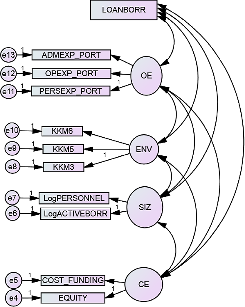
Table 8 The goodness of fit, outreach
| Items | AVE | CR |
|---|---|---|
| Capital structure | .857 | .923 |
| Size | .913 | .955 |
| Environment | .748 | .898 |
| Operating efficiency | .858 | .947 |
| Chi square (CMIN) | 418.157*** | |
| CMIN / DF | 11.947 | |
| CFI | .934 | |
| GFI | .900 | |
| NFI | .928 | |
| RMSEA | .142 |
*** p <0.01; Note: the values of factorial loads are shown in cursive
Source: author
The convergent and discriminant validity are positive; thus, we decided to develop the structural equation model. In Figures 4.a and 4.b, we show the model testing the relationship between independent variables and outreach. In these figures, we show the coefficients and significance. As shown in the case of the financial performance analysis, we found both a significant direct and indirect relationship between outreach and independent variables. Figure 4.a shows the result without environment and 4.b with it. As we see, when we add environment (KKM 3, 5 and 6), we find a negative and significant relationship with operating efficiency, and with outreach (LOANBORR). However, in this case, both the coefficient and significance of the effect of operating efficiency on outreach decreases. We validate the results of Figure 4.b in Table 9.

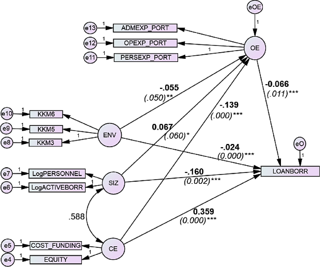
Table 9 A structural model for outreach with the environment
| OP | LOANBORR | |
| Operating efficiency (OE) | -0.066 (.011)*** | |
| Capital structure (CE) | -0.139 | 0.359 |
| (0.000) *** | (0.000)*** | |
| Size (Siz) | 0.067 | -0.160 |
| (0.060)* | (0.002)*** | |
| Environment (ENV) | -0.055 | -0.024 |
| (0.050) ** | (0.000)*** |
**: significance at 95%, *** 99%
Correlation between CE and SIZ 0.588
Source: author
We also tested the model by removing operating efficiency as a mediator variable, but coefficients and significance are very similar, as we see in Table 9.
As we note in Table 9, operating efficiency proves to be, as expected, negative and significant related with outreach, which is consistent with the results of Cull et al. (2009 y 2014), Nwachukwu (2014) and Pati (2015). Also, our result for the capital structure is both positive and significant, as stated by Cotler and Rodríguez-Oreggia (2008) and Kar (2012), but in our work, this only occurs when the effect is through operating efficiency, as opposed to a direct effect.
Regarding the size of the MFI, we find a positive and significant relationship with outreach, through operating efficiency, unlike Cull et al. (2011), Kar (2012) and Gutiérrez-Goiria et al. (2016). Finally, our results suggest that the environment has a significant adverse effect on outreach, which differs from the findings of Cull et al. (2011) and (2014).
4. Conclusions
Financial performance and outreach are two essential variables related to MFI mission drift. However, there is still no consensus regarding which variables have a significant effect on these two parameters. In this study, we address this concern. We use structural equation modeling, a technique that allows variables to be correlated with each other either directly or indirectly, to construct proxy indicators for financial performance, outreach, and for independent variables like environment (corruption, the rule of law and government inefficiency), size, capital structure, and operating efficiency.
After proving our model’s goodness-of-fit and verifying other necessary validity proofs, we did not find a direct relationship between financial performance and the independent variables. However, we found that this relationship becomes significant when we use operating efficiency as a mediator variable (i.e., personal and administrative expenses). In other words, environment (corruption, the rule of law and government inefficiency), size and capital structure maintain a significant effect on operating efficiency, which in turn affects financial performance. The latter implies that in an environment where there is corruption, a lack of the rule of law, and government inefficiencies, MFIs financial performance is lower because those independent variables have a significant effect on operating expenses. In addition, it implies that operating costs has a knock-on effect on operating performance and the adverse effects on financial performance.
Concerning outreach, we found both significant direct and indirect effects. In particular, we found an adverse effect on operating efficiency, a positive effect on capital structure, the nonexistent effect on size, and lastly adverse effect on the environment. Our results suggest that in an environment of corruption, lack of the rule of law and government inefficiency, the loans are smaller. Which suggest that, in countries with security and corruption issues low-income people are abundant. As a result, the services offered by MFIs are broader in scope. Regarding the significance of size, we found that the larger the MFI, the smaller the size of the loan, which could be a consequence of MFI risk policies to limit the size of the loan, or MFI business diversification (micro-insurance, small business loans).

