


 nueva página del texto (beta)
 Inglés (pdf)
 Artículo en XML
 Referencias del artículo
 Enviar artículo por email
 Citado por SciELO
  Similares en
SciELO
Similares en
SciELO 
 Permalink
1. Introduction
After the Second World War, the United States achieved the status of the number one economy in the world. For that reason, whatever major domestic economic or political events occur in that country, they have a significant impact beyond its borders. In the case of Canada and Mexico, its Northern and Southern neighbors, that impact is particularly noticeable due to the close commercial and cross-border investment relationships that were boosted by the North American Free Trade Agreement (NAFTA) with the USA since 1994, more than two decades ago. Geographical proximity and a shared border of approximately 3,200 kilometers in the case of Mexico and 8,891 kilometers in the case of Canada, make geopolitics a very significant component of the daily interactions among the three NAFTA countries.
Every year Mexican workers in the USA send billions of dollars as remittances to their families in Mexico1. That income represents a significant component of the recipient families’ consumption expenditure and small productive investments. As well, most of Mexico’s goods and services exports are sent to the USA. For example, in 2016 its exports to the USA totaled $302.6 billion USD, which represented 81 % of total exports (Banxico, 2017). Furthermore, many Mexican companies have business operations in the USA, enticed by the breath and depth of that country’s consumer market; and a large number of American companies operate in Mexico attracted by the low cost and high quality of labor, and the relatively large population of the country2. During the same year, Canada’s exports to the USA totaled $353.8 billion USD, or 75 % of its total merchandise exports; that means that Canada’s commercial dependence with respect to the USA is marginally lower than Mexico’s, but still highly significant.
From3 that perspective, it could have been expected that the news of the campaign trail, in particular those that implied the probability that Trump could become President of the U.S. was on the rise, given his unfavorable positions with respect to NAFTA, would affect both other member countries financial variables in a noticeable way. Nevertheless, during the campaign’s news affected mostly the Mexican financial markets, and the Canadian markets very scantly. That fact was the main motivation for this work considering that, even when the Canadian and the Mexican economies are not so different in absolute size, nor in terms of the economic importance represented by foreign trade with the U.S. relative to total GDP, only one of the two experienced significant responses in the stock market index and the currency exchange rate to the campaign news.
A better understanding of the influence of the campaign trail events, proxied by electoral polls and bets, on the evolution of the Canadian and the Mexican financial markets is of much interest for financial economists, policy designers and investors.
For many decades, scientific polls and prediction markets have been extensively studied and those results have been published in the political science literature (Hillygus, 2011; Graefe, 2014; Graefe, et al., 2014; Rhode Strumpf, 2004). Most studies that establish a relationship between politics and financial variables have focused on electoral processes and domestic stock markets (Jones Banning, 2009; Białkowski, Gottschalk, Wisniewski, 2008; Chien, Mayer, Wang, 2014; Döpke Pierdzioch, 2006; Forsythe, Rietz, Ross, 1999; Hung, 2013). However, to our knowledge, no studies have explored how does an election campaign that takes place in one country affect the financial markets of a third country. This paper uses the prediction markets quotes and the publicly disseminated scientific polls produced during the 2015-2016 USA Presidential campaign4, to determine the nature and intensity of their influence on Canada’s and Mexico’s currency exchange rate quotations and stock market indices performance.
The main hypothesis of this work is that the Mexican stock market and exchange rate were more affected by the electoral process news than the Canadian stock market and exchange rate, revealing a greater vulnerability/dependence of Mexico’s markets to external events. More specifically, what appeared to be anecdotal evidence of the Mexican financial variables hypersensitivity to announcements and reports that the Republican candidate was making progress among voters is here documented and statistically tested to prove that, by contrast with Canadian financial variables, the former were much more reactive.
The data on voters’ preferences used in this analysis was retrieved from two main sources: the Iowa Electronic Markets (IEM) for bets on the outcome of the election (henceforth referred to as the “prediction market results”), and data from FiveThirtyEight for the USA national polls on the 2015-2016 Presidential campaign. The Mexican Stock exchange prices are represented by the Mexican index IPC, the Mexican exchange rate is quoted as Mexican pesos per US dollar; the Canadian stock market performance is proxied by the Toronto Stock Exchange Index (TSX) and the country’s currency exchange rate is expressed as Canadian dollars per US dollar. All the economic variables were retrieved from Bloomberg information services databases.
The results obtained from Johansen’s (1988) Cointegration Tests, the Vector Error Correction Models (VECM) and the Vector Auto Regression Models (VAR), suggest that prediction markets information contemporaneously affects both Mexican series (IPC and MXNUSD) while polls information disseminates at a slower speed and has a lagged effect of one day. In addition, in both cases, the possibility of the Democratic candidate winning the presidency has a positive effect in both the IPC and the MXNUSD. Supporting our initial hypothesis, results also show that Canadian series are not affected by the expected outcome of the 2015-2016 USA Presidential Election.
While this study is limited to the analysis of only two financial variables (stock market indices and currency exchange rates), other several issues related to the influence of the U.S. electoral process over other countries markets remain attractive subjects of further study. For instance, the analysis may extend to measure the impact that the news on the voters’ preferences had on specific industries, firms, or other financial variables both in Canada and Mexico, and beyond NAFTA (e.g. other Latin American countries, E.U. countries, Russia, etc.). Also, depending on the outcome of the initiatives of Trump on the revision of NAFTA, the building of the border wall, or on the outcome of the ongoing probe on Trump campaign’s contact with Russian officials, may produce interesting objects of study.
The next section refers to some of the most notorious events that took place during the 2015-2016 USA Presidential campaign, and briefly discusses some well-accepted theories on the determination of currency exchange rates and stock market prices. The third section reviews the literature on scientific polls and prediction markets. The fourth section presents the data, the econometric methodology applied and the interpretation of the results obtained. The last section contains some concluding remarks.
2. The 2015-2016 U.S. Presidential Campaign, Generally Accepted Financial Markets Theories, and How Are They Related
The U.S. 2015-2016 Presidential campaign surprisingly revealed that, beyond an intensive international trade and investment activity, another powerful link exists among NAFTA member countries. The noticeable effects that campaign had on Mexican financial markets (and, to a much lesser extent, on Canadian financial markets), suggest that the events taking place in the political arena contaminated financial markets. As the electoral process developed, Donald Trump was elected by the Republican Party as Presidential Candidate on May 26th, 2016, and former Secretary of State Hillary Clinton was elected as the Democratic candidate one month later, on June 6th, 2016.
Since the beginning of the preliminary campaign to obtain the nomination of the Republican Party, Trump expressed his concern that millions of foreign citizens (mostly Mexican nationals) live and work in the USA without proper government authorization, and he pledged to expulse them from the U.S. territory. He promised to build a thousand of kilometers-long wall, along the U.S.-Mexico border to stop illegal immigration and drug smuggling. He also frequently said that he would seriously consider the termination of NAFTA in case a comprehensive revision could not make it more “fair” to the U.S. During his campaign speeches, he repeatedly mentioned that NAFTA was the “worst trade agreement ever negotiated by the USA” and expressed that it could be blamed for the extensive unemployment observed in several mid-West states of the U.S. The public speeches in which Trump expressed negative opinions about Mexico5 consistently had negative effects on that country’s currency exchange rate and on the performance of its stock market. By contrast, the commentaries of Clinton, the Democratic contender, were much friendlier and positive towards Mexico, and had an exactly opposite effect on those two variables. The effects of both contenders’ speeches on Canadian financial variables were much less noticeable, and may be considered negligible, as will become evident from the results of the econometric analysis presented in the following sections of this paper.
As the electoral process developed, Trump was first elected by the Republican Party as Presidential Candidate (on May 26th, 2016), and then, former Clinton was elected as the Democratic candidate (one month later, on June 6th 2016). All throughout the campaign6, the predictive markets had an active betting activity on its outcome contracts, and many polls were published daily on the same subject.
Once the Presidential campaign started, more often than not, when Trump’s campaign made any progress, the Mexican currency depreciated vis à vis the USD, and the IPC had a negative performance, but when Clinton’s electoral chances seemed improved, the opposite was true. As mentioned before, the effects over the corresponding Canadian variables were much less noticeable.
On a theoretical perspective, the differentiated response of the MXNUSD and the CADUSD response, and of Canada’s and Mexico’s stock markets to the campaign’s events is an interesting case that can be interpreted under the tenants of the Efficient Markets Hypothesis (EMH). This is a topic that has not been studied before, and that opens a whole new perspective on how two important domestic financial variables are influenced by the events taking place in the political arena of a third country.
From a rudimentary stage at the beginning of the 20th century, through the decades, the underlying knowledge-body of polls, modern statistical theory has gained full scientific status. To the present, polls are widely used in many areas of the social sciences with considerable success. In what concerns the USA’s Presidential elections, polls on citizens’ intention of vote if the election took place on a particular day are always of great interest to all groups of society. As discussed in the third section of this work, numerous studies have attempted to determine their importance, and test their reliability.
During the early years of the 21st century, betting markets, also known as “prediction markets”,7started trading “contracts whose payoff depends on unknown future events” (Wolfers Zitzewitz, 2004). Underlying the activities of predictive markets is the purpose to create a mechanism through which the subjectivity and beliefs of participants are reflected on a contract’s prices and, in that sense, become measurable. These contracts on very different types of outcomes offer a certain payoff to those agents that make the right predictions. In effect, the Presidential election outcome contract is one notable representative of that universe. On Wednesday, November 19th, 2014, at 11:30am CST, the Iowa Electronic Market (IEM) started trading a winner-takes-all contract based on the outcome of the 2016 USA Presidential election, which this study utilizes to infer electoral preferences.
The Efficient Markets Hypothesis (EMH), postulated by Fama (1970, 1991), gives a theoretical explanation of the drivers of public companies’ stock prices and the currency exchange rate markets. At the same time, information on the Presidential election campaign trends was reflected in the polls reports and the prediction markets quotes. A relevant question that immediately arises- and this study addresses- is whether the former’s or the latter’s signals were efficiently incorporated in the two financial variables of interest, and in case the answer is positive, which one preceded the other.
3. Traditional Theories on the Determination of Currency Exchange Rates and Stock Prices of Publicly Traded Firms
The number of published studies that attempt to explain how does the determination of currency exchange rates takes place is vast. There is a strong motivation for that: firms and individuals who are exposed to exchange rates fluctuations have a clear motivation to find ways to anticipate the future value of exchange rates. From the perspective of the treasurer of a Multinational Corporation or an international investor, anticipated knowledge of the future of the exchange rates would minimize their exposure, and possibly generate extraordinary profits.
Different theoretical proposals, supported by rigorous economic arguments have been developed for many decades. Some are very intuitive and logical, but hardly any of them has been tested and empirically confirmed. There are three popular and well-known conceptions that explain the exchange rates determination, based on which different variations and extensions have been developed, although here we only refer to the original approaches.
The first one is known as the Purchasing Power Parity (PPP), proposed by the Swedish economist Gustav Cassel (Cassel, 1918). This theory suggests that the exchange rate between the currencies of two countries should be equal to the ratio of those countries’ price levels. The second theory is called the Interest Rate Parity (IRP) and was proposed by John Maynard Keynes (Keynes, 1924). It states that the differences between the interest rates of two countries should be equal to the spread (differential) between the forward and spot currency exchange rates. The third very well-known exchange rate determination theory is the International Fisher Effect (Fisher, 1930), that says that the nominal exchange rate between two countries should change by an amount similar to the difference between the domestic rates of inflation of those countries, so as to maintain a constant real rate of return in all countries.
All three theoretical approaches rely on the assumption that arbitrage opportunities may not exist and, for that reason, international markets are in equilibrium. As well, all three have been repeatedly tested but, except for IRP, very little empirical evidence supports them. So, a generally accepted conclusion is that no single model provides an adequate explanation of most of the movements in nominal and real exchange rates under a floating exchange rate regime (Mussa, 1984), leaving open the possibility to explain the evolution of currency exchange rates by other factors such as changes in perception and expectations of agents. Likewise, the behavior of stock prices traded in public markets has long been studied in the academic literature, and one of the major contributions to better understand it is the EMH, proposed by Fama (1970, 1991). The EMH postulates that an equilibrium price remains until new information is incorporated to the original information set. The market will interpret it and reformulate the asset’s worth appraisal, thus, modifying the equilibrium price.
According to Dyckman and Morse (1986) “information...is reflected by security prices when prices change because of changes in demand. The process of disseminating and analyzing information to develop new expectations about future prices determines the degree of efficiency in the market”. The result of the new appraisal of the asset’s worth might as well be an increase or a decrease of its market price. The price variation will depend in direction and magnitude on the investors’ interpretation of the information relevance and sense, in terms of risk and future returns. Accordingly, the new equilibrium price will hold until yet another piece of relevant information reaches the market. Elton and Gruber (1991) neatly express this idea: "When someone refers to Efficient Capital Markets, they mean that security prices fully reflect all available information."
The EMH hypothesis provides the grounds to explain why, during the U.S. Presidential election process, the Mexican stock market behavior and the currency exchange rate had an immediate positive reaction to the news of Clinton’s advances in the polls, whereas the opposite effect happened when Trump’s position improved. The sensitivity of the Canadian variables was milder, even when the political implications of one candidate or the other winning the Presidential election potentially represented important differences for Canada. No doubt, this asymmetry of response poses an interesting theoretical question that we address in the last of the paper.
4. Literature Review
Traditionally, the generally accepted measure of the subjective probability on the outcome of political elections has been the opinion polls reported results. However, in more recent times, prediction markets have been increasingly followed by many interested parties as reliable sources of the market “sentiment” regarding intention of vote8. This section briefly reviews a sample of works on what the academic literature has reported on both.
Public opinion polls have long played an important role in the daily follow-up and the ex-post study of political elections (Hillygus, 2011). Scientific polling, introduced in 1936, consists on asking to a random sample of respondents who would they vote for, if the election was held on that day. Polls do not provide predictions, but snapshots of public opinion at given points in time; however, there are reasons to believe that they have been an influential component in the American elections outcomes of recent history (Graefe, 2014).
Political polls were initially published in the Literary Digest, an American magazine founded in 1890. It was the largest and best-known nonscientific survey, which tabulated millions of returned postcard ballots that were mass mailed to a sample drawn from telephone directories and automobile registries (Rhode Strumpf, 2004). The weekly magazine used to conduct a straw poll regarding the likely outcome of presidential elections. It always predicted the winner for the 1920, 1924, 1928 and 1932 elections.
However, that was not the case for the 1936 USA presidential election. In that year, the Literary Digest poll concluded that the Republican candidate, Governor Alfred Landon, was the likely winner. Paradoxically, Mr. Landon only won two states, while President Franklin D. Roosevelt won the other 46 states. This failed prediction meant the disappearance of the Literary Digest, despite its former successful track (Squire, 1988).
The failed prediction might have been due to the nature of the sample used by the magazine. There might have been a sample and a response bias, since the polled groups were mainly Digest’s readers, automobile owners, and telephone users (Squire, 1988). Americans belonging to those groups were mostly Republicans and had an income that was slightly above the national average because they could afford to pay a weekly magazine, have a car, and pay telephone bills during the difficult times of the Great Depression (Gallup, 1972). Remarkably, there was a scientific poll conducted by George Gallup during the 1932 election period which, not only predicted the right winner, but also predicted that the Literary Digest results would be totally wrong. Interestingly enough, Gallup was one of the pioneers of survey sampling techniques.
The Gallup poll represented a significant scientific enhancement of polling techniques. Scientific polls became the mainstream and have become an integral part of any Presidential election campaign in the USA. They are the basis for campaign strategy by candidates, parties, and interested groups, and they are a primary tool used by academicians and journalists to understand voting trends and voter’s behavior (Hillygus, 2011). Since 1936 and until 2008, the Gallup poll correctly predicted the winner of the USA Presidential elections.
However, at the time of the 2008 election, a poll analyst, Nate Silver, found that the Gallup poll was ranked in the last spots of accuracy, compared to other polling firms. Competition among polling firms had arrived and was to improve the quality of results. For instance, FiveThirtyEight is a polling aggregation website founded, precisely, by Nate Silver in 2008. The methodology used by Silver basically consists in balancing out the polls with comparative demographic data. Even though the results obtained by the webpage is just the reprocessing and the analysis of polls made by others, FiveThirtyEight has rapidly become quite popular and has won numerous awards.
What can be said about scientific polls is that their statistical foundations are still in a process of gradual but consistent improvement and, while no polling service (including FiveThirtyEight) can claim a flawless record, they are all increasingly scientific and robust, and can produce reasonably good forecasts.
Prediction markets, also called “information market” or “event futures con-tracts” allow participants to trade in contracts whose payoff depends on unknown future events (Wolfers Zitzewitz, 2004). Hence, market prices move in response to what investors believe the outcome of a particular event will be.
There are several prediction markets. For instance, the market based on the Hollywood Stock Exchange, where participants trade movies and actors, speculate on when films will have their opening dates, and box office returns, among others. A former popular webpage was TradeSports (that used to trade contracts on different sports -American football, basketball, golf- matches outcomes), however it does no longer exists. Nowadays, the most popular prediction markets are the ones from Iowa Electronic Markets, where contracts on predictions of USA elections, earnings and returns markets are traded.
The Iowa Electronic Markets (IEM) was created for teaching and research purposes by the University of Iowa in 1988, and eventually became a commercial entity. In it, traders buy and sell real-money contracts based on their beliefs about the outcome of an election or other types of events, and the price of a contract can be interpreted as a forecast of the outcome (Iowa Electronic Markets, 2017). One of the most popular contract types traded at the IEM is the “winner-takes-all” contract, which reveals the market expectations of the probability that certain event occurs. The contract is like a “state” price that pays one dollar if a given event occurs, and zero dollars if it does not. Particularly, in the case of the 2016 USA Presidential election, the winner-takes-all market contract was based on the popular vote received by the official Democratic and Republican nominees.
Betting on the USA Presidential election is not a new phenomenon. A large, active and highly public market for betting on elections has existed over much of that country’s electoral history, as far back as the XIX Century. The center of the betting activity in the country was located in New York. Those betting markets were widely recognized for their remarkable ability to predict election outcomes (Rhode Strumpf, 2004).
Betting markets had high predictive power in the four elections that took place from 1884 to 1896. According to records of the time, market participants perceived those electoral processes as “very close”. Also during the elections of reference, newspapers like the New York Times reported daily quotes from October until the Election Day. The 1916 election showed how important betting markets were: bets in New York for that year were around the equivalent of $165 million of year 2002 dollars (Rhode Strumpf, 2004).
A contributing factor for the large size of betting markets is that, before the mid-1930s, there were no scientific polls that could aggregate information the way those markets did. But once both existed, there has been a debate about which one has more predictive power. Hence, several studies have compared the accuracy of both methods to forecast elections results.
Studies where the performance of both markets has been evaluated by comparing their daily market forecasts, indicate predictive markets prove to be more accurate (Graefe, 2014). This can be explained by the fact that polls are seen more like people’s perceptions on that particular day, while market makers are supposed to trade according to expectations and careful analysis of the possible outcomes odds.
Yassin Hevner (2011) tested the accuracy of prediction markets using prices from the IEM. According to their results, prices have been more accurate than polls more than 75 % of the time since 1988. Polls had 2.1 % points of average absolute error in forecasting elections, compared to only 1.5 % points in the case of market prices.
The greater accuracy attributable to prediction markets might be explained by the fact that trading dynamics (and the wide variety of participant agents) in the market cancel out individual biases and errors (i.e., publicly open markets are “efficient”) (Yassin Hevner, 2011). However, that same characteristic may also represent a source of bias, because the traders that participate are supposed to make informed judgments. However, information cascades can affect them; i.e., participants might be affected by “herd behavior”, where buy or sell decisions are heavily influenced by the observed actions of other market participants (Anderson Holt, 1997). This can negatively affect prediction market forecasts due to unexpected spikes in prices.
In addition, markets can also be affected by their traders’ characteristics. Usually they are young, male, well-educated and earn high incomes, but that might not be representative of likely voters, as was the case during the 1936 USA Presidential election, where a bias on the poll participants sample was the main cause of the wrong predictions published by the Literary Digest (Berg et al., 2001).
Interestingly, Rothschild (2009) corrected polls and prices for inherent biases, and his results also support the conclusion that prediction markets outperform polls, both at the beginning of campaigns, and all along the races. Again, the reason might be that market price setters can act on electoral factors that are not incorporated in polls until the next poll (Erikson Wlezien, 2012).
Hence, due to the quicker reaction capacity they have compared to polls, prediction market prices are expected to reflect Election Day fundamentals that are not yet incorporated in the polls. This is clearly one advantage of predictive markets, especially when there are periods of high intensity of information flows.
Notwithstanding, Erikson and Wlezien’s (2012) study, where election markets’ accuracy was assessed in years before and after the introduction of opinion polling, concludes that prices of prediction markets add nothing to election prediction beyond polls. Probably because after scientific polls began to be commonly used, betting markets were relegated and became heavily dependent on what polls showed, even if the latter were not very accurate.
Graefe et al. (2014) found that using polls from PollyVote provided more accurate forecasts in the six elections that they evaluated. They also mention that for the elections that took place between 1992 and 2012, the PollyVote forecast was 7 % more accurate than the Iowa Electronic Markets 7-day average, a subtlety that could represent an interesting area of research.
Using Granger causality tests, Duquette et al. (2014) conclude that during the 2012 USA Presidential election, polls anticipated InTrade prediction market prices. This could be interpreted as traders in prediction markets making their investments decisions based on respondents’ intentions of vote, even if the latter can provide inaccurate information about preferences9. These seemingly contradictory evidences are difficult to reconcile because, even when prediction markets work on continuous real time, and polls are taken only at discrete points in time, polls performance evaluation also shows satisfactory results.
Besides, there is also a problem of comparison: market prices reflect continuous forecasts of the expected vote, while polls register the vote intentions only at the time those polls were taken (Erikson Wlezien, 2012). However, when polls are converted into forecasts based on their historical relationship with the vote, they can sometimes beat market prices as predictors. For example, poll projections take into account historical records of polls to make forecasts. This can be done by regressing the candidate’s share of the vote on her polling results during certain time period before the election date (Graefe, 2014). Using poll projections, Berg, Nelson, and Rietz (2008) found that they were more accurate than prediction market prices.
Another methodological approach is that of “poll averages”, which reflect small bits of information that might go unnoticed by most traders (Duquette et al., 2014), hence contributing to poll’s accuracy. Graefe (2014) compared three different poll-based forecasts: polls published on a particular day, polls’ average on a seven-day period and poll projections, using polls conducted within 100 days prior to each of the 16 elections from 1952 to 2012, and compared them with the IEMs’ vote-share market (a combined forecast of all market participants). The comparison indicated that single polls predicted the correct winner 79 % of the time, combined (averaged) polls were accurate by 86 %, and poll projections were accurate 88 % of the time. With a 79 % accuracy record, prediction markets were comparable only to single polls (Graefe, 2014).
However, when polls from different firms are aggregated, potential biases introduced by individual firms’ methodologies can affect results. Volatility might be reduced and, in that sense, combining is a useful approach to reduce forecast error, but accuracy might not be improved (Hillygus, 2011).
Combining might also be helpful for prediction markets. When seven-day averages of IEM contract prices were compared to their original prices in each election from 1992 to 2012, the averages were more accurate forecasts (Graefe et al., 2014). This result is in apparent contradiction to the EMH, which states that asset prices reflect all relevant information and thus provide the best prediction of future events given current information (Roll, 1984). If averages of prediction markets proved to be more accurate than daily prices, these markets are not truly efficient in the informational sense, at least from 1992 to 2012. By contrast, analyzing the outcome of elections from 1868 to 1940, Rhode and Strumpf (2004) found that there was a violation of the arbitrage-free condition for the elections between 1912 and 1916. He concluded that, since efficient prices of election markets should reflect the probabilities of election outcomes, there is no possibility of making gains through arbitrage operations. Again, conflicting results suggest there may be methodological issues that distort a direct comparison of the alternatives.
Consequently, we conclude that to focus on the empirical evidence at hand, both polls and prediction markets data can be used interchangeably as measures of the subjective probabilities of a Republican or a Democratic winner on the 2016 USA Presidential election. While our work does not represent a contribution to the attempts to clarify which of the two is more reliable, we do find these ex-ante predictors were highly significant in explaining the behavior of the IPC Index and the MXN/USD during the campaign period, and not in the case of the TSX and the CADUSD.
5. Research Design and Empirical Findings
This work hypothesizes that market participants interpreted the potential out-comes of the U.S. 2016 Presidential Election as either headwinds or tailwinds for the U.S.’s NAFTA partners, and that the intensity of their impact was differentiated among the other two countries. The success of Mrs. Clinton, the Democratic candidate representing the status quo, would have implied tailwinds for Mexico and Canada. The triumph of Mr. Trump, the Republican candidate, representing a nationalistic and protectionist view of the world would, on the contrary, imply headwinds for both countries. The expectation was that the potentially negative effects would be stronger for Mexico, as Mr. Trump’s protectionist rhetoric reiteratively targeted that country’s exports as a threat to employment in many regions and industries of the USA economy.
The development of the Presidential campaign represented frequent ups and downs in the preferences of voters for both candidates. A naive observation of their effect on the performance of the stock market and the exchange rates of Mexico and Canada suggested a more formal analysis could be very interesting.
Two alternative sources of information were selected to capture the preferences of U.S. voters during the months leading to the USA Presidential Election day on November 8th, 2016. Due to their dynamic nature and fast update, the data on “bets” and “polls” on the likely outcome of the election were used to capture the trends in voters’ preferences towards the two front-runner Presidential candidates. The bets market was data represented by the IEM prediction market “winner-takes-all” (WTA) contracts, and the polls data corresponded to the daily summary of polls10 collected and reported by the FiveThirtyEight service. In addition, Mexico’s and Canada’s currency exchange rates and stock market indices were used as dependent variables.
6. Prediction Market Data
On Wednesday, November 19, 2014, at 11:30am CST, the IEM started trading a winner-takes-all contract on the 2016 USA Presidential election11. The payoffs in this market were referenced to the popular vote received by the official Democratic and Republican nominees in the 2016 USA Presidential election. Payoffs were not affected by votes received by nominees from other parties, the outcome of the Electoral College, or any vote taken by the House of Representatives should such a vote be necessary.
The prediction contracts of interest to this study include the following two:
DEM16_W T A: $1 if the Democratic Party nominee receives the majority of popular votes cast for the two major parties in the 2016 USA Presidential election, $0 otherwise
REP 16_W T A: $1 if the Republican Party nominee receives the majority of popular votes cast for the two major parties in the 2016 USA Presidential election, $0 otherwise
The two contracts are dependent on one another (as DEM16_WTA increases, REP16_WTA decreases). Hence, to operationalize these variables, they were combined into a new variable. This avoids the potential multicollinearity, a problem that would increases the Variance Inflation Factor (VIF)12 of the model. Since both variables have the same units, calculating their spread is an acceptable solution. The daily spread between the Last Price of both contract types (DEM16_WTAt - REP16_WTAt) was labeled as DEMREP_BETt.
7. Aggregated Polls Data
The data on aggregated polls was retrieved from the FiveThirtyEight service13. This entity collects the output from 1,106 National Polls on the 2016 USA Presidential election forecasts. The polls have different frequency of publication but, on any day, dozens of polls results are combined and reported by FiveThirt-yEight. Based on the outcome of each poll, FiveThirtyEight estimates a share percentage of intention of vote for each one of the candidates, which is then adjusted for likely voters, omitted third parties, trend line and house effects. It is important to notice that the share of voters assigned to Presidential candidates by each poll is also dependent on one another, just as in the case of the contract prices of the IEM. At the same time, the theoretical minimum in each case is also 0, hence a spread between them to include both data series in a single variable was calculated as follows: (adjpollClintont - adjpollTrumpt). The new variable was labeled DEMREP P OLLt:
Data from polls are not published as frequently as the IEM contracts prices, especially those further away from the election date. However, after April 19th, 2016, once both candidates won their New York primaries, data series of polls are much more complete. Hence, we use that as our starting date for the models that include them. In the time-period sample between bets and polls, they have a 70 % correlation which indicates a close relationship between them.
8. Financial Markets Variables
The market variables of interest are the main equity stock market indices of Mexico and Canada (IPC and TSX respectively), and their currency exchange rates versus the U.S. dollar (MXNUSD and CADUSD, respectively). All series were retrieved from Bloomberg’s database with daily frequency for the period 11/18/2014 to 11/10/2016. Data on the MXNUSD is quoted as the quantity of Mexican pesos per U.S. dollar; the same applies for the CADUSD, quoted as the quantity of Canadian dollars per U.S. dollar. The variables were log-transformed and their first-differences were obtained.
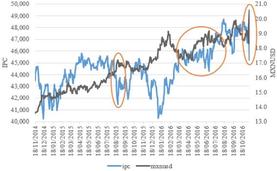
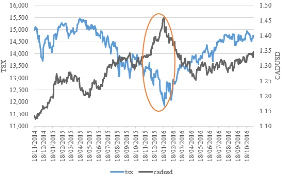
Figure 1 represents Mexico’s main stock index and the MXNUSD exchange rate. Most of the time, when the IPC recorded negative returns, the Mexican peso lost value against the US dollar. Both variables suffered negative effects after the first Republican debate occur in August of 2015 when Trump claimed that “Mexican government was purposely sending immigrants (“the bad ones”) into the United States” (Shear, 2015). These variables were also greatly affected towards the end of 2015 and beginning of 2016. When there was an increased expectation that the Federal Reserve would raise interest rates, which ultimately did happen. This decision affected both Mexican and Canadian variables (see Figure 2). From March 2016 on, the volatility of Mexican financial variables surged, since during that time Trump remained the front-runner throughout the Republican primaries, and was finally chosen as the Republican candidate. However, the most dramatic negative effect for Mexican financial markets occurred after the Election Day when the MXN move from $18.32 MXN per USD to $20.57 MXN per USD, i.e., approximately 12 %, in a matter of a few hours.
The sample period includes two days after the U.S. Presidential Election (Nov 9th and 10th 2016) to capture the immediate post-election results effect on the variables of interest. For that purpose, the DEMREP_BETt and DEM-REP_POLLt data for those dates was represented by including a value of -1 in each, to indicate the actual result of the election: Trump being elected over Clinton. Tables 1 and 2 below, present the descriptive statistics of the financial variables of this study.
Table 1 Descriptive Data of IPC and MXNUSD in levels and in log-returns.
| IPC | MXNUSD | LRIPC | LRMXNUSD | ||
|---|---|---|---|---|---|
| Mean | 44,614.24 | 16.89 | Mean | 0.00 | 0.00 |
| Median | 44,698.01 | 16.89 | Median | 0.00 | 0.00 |
| Maximum | 48,694.90 | 20.58 | Maximum | 0.04 | 0.08 |
| Minimum | 40,225.08 | 13.56 | Minimum | -0.05 | -0.03 |
| Std. Dev. | 1,821.97 | 1.56 | Std. Dev. | 0.01 | 0.01 |
| Skewness | 0.0865 | -0.0978 | Skewness | -0.3111 | 1.4466 |
| Kurtosis | 2.6549 | 1.8511 | Kurtosis | 5.3807 | 15.3601 |
| Jarque-Bera | 3.10 | 28.24 | Jarque-Bera | 125.64 | 3343.74 |
| Probability | 0.2124 | 0.0000 | Probability | 0.0000 | 0.0000 |
| Observations | 499 | 499 | Observations | 498 | 498 |
| Correlation | IPC | MXNUSD | Correlation | LRIPC | LRMXNUSD |
| IPC | 1.00000 | 0.49607 | LRIPC | 1.00000 | -0.50326 |
| MXNUSD | 0.49607 | 1.00000 | LRMXNUSD | -0.50326 | 1.00000 |
Source: Own elaboration.
Table 2 Descriptive Data of TSX and CADUSD in levels and in log-returns.
| TSX | CADUSD | LRTSX | LRCADUSD | ||
|---|---|---|---|---|---|
| Mean | 14,145.70 | 1.29 | Mean | 0.00 | 0.00 |
| Median | 14,308.93 | 1.30 | Median | 0.00 | 0.00 |
| Maximum | 15,450.87 | 1.46 | Maximum | 0.03 | 0.02 |
| Minimum | 11,843.11 | 1.12 | Minimum | -0.03 | -0.02 |
| Std. Dev. | 801.74 | 0.06 | Std. Dev. | 0.01 | 0.01 |
| Skewness | -0.5782 | -0.3193 | Skewness | -0.2348 | -0.1171 |
| Kurtosis | 2.6066 | 3.4729 | Kurtosis | 4.1333 | 3.5192 |
| Jarque-Bera | 30.96 | 13.10 | Jarque-Bera | 31.16 | 6.72 |
| Probability | 0.0000 | 0.0014 | Probability | 0.0000 | 0.0347 |
| Observations | 498 | 498 | Observations | 497 | 497 |
| Correlation | TSX | CADUSD | Correlation | LRTSX | LRCADUSD |
| TSX | 1.00000 | -0.70422 | LRTSX | 1.00000 | 0.39186 |
| CADUSD | -0.70422 | 1.00000 | LRCADUSD | -0.39186 | 1.00000 |
Source: Own elaboration
The econometric analysis of the impact of voters’ preferences during the 2016 USA Presidential campaign over the evolution of the financial markets of Canada and Mexico is performed using a Vector Auto Regression (VAR) approach.
As a first step in the analysis, the variables (and their returns) are tested for stationarity, as the utilization of non-stationary variables for regression analysis may produce spurious results. Table 3 shows Augmented Dickey-Fuller (ADF) tests to determine the presence of unit roots in the financial variables of both countries. The results of the ADF tests for the financial variables in levels (log-prices) and their first-differences (log-returns) indicate that the four variables are I(1) in levels, but I(0) in first differences. The polls and prediction market variables are, by default, stationary, as their range of possible values is within +1 and -1.
Table 3 Augmented Dickey-Fuller Tests.
| Variable | Log-prices | Log-returns |
|---|---|---|
| IPC | 0.0625 | 0.0000 |
| MXNUSD | 0.6659 | 0.0000 |
| TSX | 0.2987 | 0.0000 |
| CADUSD | 0.1063 | 0.0000 |
Note: The probabilities are based on MacKinnon (1996) one-sided p-values.
Table 4 shows the results of the Johansen Cointegration Tests for the Canadian and Mexican financial variables, for a linear deterministic trend (i.e., with intercept in the cointegrating vector). The cointegration tests results for the Mexican LIPC and the LMXNUSD indicate the existence of one cointegrating vector according to both, the Trace p-value test and the maximum eigenvalue test. Surprisingly, no cointegrating relationship is detected for the Canadian LTSX and the LCADUSD in neither of the two cointegration tests.
Table 4 Johansen Cointegration Tests.
| Variable | CE’s | Trace p-val | Max-eign p-val |
|---|---|---|---|
| LIPC | None* | 0.0313 | 0.0263 |
| LMXNUSD | At most 1 | 0.3621 | 0.3621 |
| LTSX | None | 0.2024 | 0.5095 |
| LCADUSD | At most 1* | 0.0376 | 0.0376 |
Source: Own elaboration
When variables are cointegrated, the right specification is a Vector Error Correction Model (VECM). Accordingly, to estimate the Mexican financial variables response to the electoral preferences, a VECM model that incorporates the existence of a long-term relationship (cointegration) is in order, as represented in equations [1] and [2] below. In the case of the Canadian financial variables, for which no cointegration relationship was detected, a VAR approach is used, as represented in equations [3] and [4].
The DEMREPit variable alternatively represents the “bets” (prediction market contract prices) time-series, or the “polls” time-series, since both were alternatively used as exogenous variables14. Contemporaneous and lagged effects of the DEMREPit variables were tested given that their signal might not be reflected on the market the same day they are published, especially, for example, in the case of some polls that were published only after the market was closed.
VECM Equations for Mexican variables:
VAR Equations for Canadian variables:
The lag order selection criteria for both models was obtained and is reported below. All the length of lag criteria indicate that one lag is optimal in the case of the LRIPC and LRMXNUSD model. In the case of the LRSTX and LRCA-DUSD the optimal lag according to the information criteria is zero. However, we implement a one lag basic model in this case too since the values of the criteria are very close, as shown in Table 5.
Table 5 VAR Lag Order Selection Criteria.
| Exogenous variables: C | ||||||
| Sample: 11/18/2014 11/10/2016 | ||||||
| Included observations: 490 | ||||||
| Endogenous variables: | ||||||
| LRIPC LRMXNUSD | ||||||
| Lag | LogL | LR | FPE | AIC | SC | HQ |
| 0 | 3298.288 | NA | 4.92e-09 | -13.45424 | -13.43712 | -13.44751 |
| 1 | 3318.202 | 39.58446* | 4.61e-09* | -13.51919* | -13.46783* | -13.49902* |
| 2 | 3320.215 | 3.985049 | 4.65e-09 | -13.51108 | -13.42548 | -13.47747 |
| 3 | 3323.401 | 6.279889 | 4.66e-09 | -13.50776 | -13.38792 | -13.46069 |
| 4 | 3327.976 | 8.983032 | 4.65e-09 | -13.51011 | -13.35603 | -13.44960 |
| 5 | 3331.972 | 7.812345 | 4.65e-09 | -13.51009 | -13.32177 | -13.43613 |
| 6 | 3332.888 | 1.783097 | 4.71e-09 | -13.49750 | -13.27494 | -13.41010 |
| 7 | 3333.137 | 0.482550 | 4.78e-09 | -13.48219 | -13.22539 | -13.38134 |
| 8 | 3333.801 | 1.281487 | 4.85e-09 | -13.46857 | -13.17753 | -13.35427 |
| Endogenous variables: | ||||||
| LRTSX LRCANUSD | ||||||
| Lag | LogL | LR | FPE | AIC | SC | HQ |
| 0 | 3476.574 | NA* | 2.31e-09* | -14.21094* | -14.19379* | -14.20420* |
| 1 | 3480.457 | 7.717912 | 2.31e-09 | -14.21046 | -14.15902 | -14.19025 |
| 2 | 3480.880 | 0.838012 | 2.34e-09 | -14.19583 | -14.11009 | -14.16215 |
| 3 | 3482.503 | 3.200361 | 2.37e-09 | -14.18611 | -14.06608 | -14.13896 |
| 4 | 3485.181 | 5.256123 | 2.38e-09 | -14.18070 | -14.02638 | -14.12009 |
| 5 | 3489.346 | 8.142872 | 2.38e-09 | -14.18137 | -14.99276 | -14.10729 |
| 6 | 3492.932 | 6.982636 | 2.38e-09 | -14.17968 | -13.95678 | -14.09213 |
| 7 | 3494.178 | 2.415638 | 2.41e-09 | -14.16842 | -13.91122 | -14.06740 |
| 8 | 3496.923 | 5.297881 | 2.42e-09 | -14.16328 | -13.87179 | -14.04879 |
* indicates lag order selected by the criterion
LR: sequential modified LR test statistic (each test at 5 % level)
FPE: Final prediction error
AIC: Akaike information criterion
SC: Schwarz information criterion
HQ: Hannan-Quinn information criterion
Table 6 shows the output of the estimation of the two VECM models on the Mexican financial variables (equations [1] and [2]). The conclusions of both analyses are the same, even though the time-period of the second VECM is shorter due to the limited availability of polls’ data. The “bets” time-series was significant for both LRIPC and LRMXNUSD contemporaneously (DEMREP_BETt). The “polls” time-series was significant in both cases with a lag of one-day (DEMREP_POLLt- 1), suggesting that polls’ (FiveThirtyEight) information is a bit slower to disseminate onto the Mexican financial variables than the betting markets’ (IEM) information. But, except for that, both have the same sign and are statistically significant, i.e., they have the same interpretation. A positive spread in the expectations of the Democratic candidate winning the election has a positive sign for the IPC equation (the stock market rallies), and has a negative sign for the MXNUSD equation (the peso exchange rate appreciates relative to the dollar). These effects were confirmed during the post-electoral period effects when, after the Republican candidate’s surprise win, the IPC had negative returns and the peso depreciated relative to the dollar. Other interesting findings in Table 5 include the fact that the cointegrating equation is significant in all cases, and that the lagged exchange rate seems to affect the stock market but not the other way around. Both are significant and their signs match our expectations.
Table 6 VECMs for the LRIPC and LRMXNUSD pair.
| Equation | Variable | Bets | Polls |
|---|---|---|---|
| Coint. Eq. (CE) | LIPC-c1 | 1.0000 | 1.0000 |
| LMXNUSD-1 | 0.0572 | -0.5740*** | |
| C | -10.8665 | -9.0736 | |
| LRIPC | CE | -0.0507*** | -0.1007*** |
| LRIPC-1 | 0.0149 | -0.0313 | |
| LRMXNUSD-1 | -0.2489*** | -0.3054*** | |
| C | -0.0025*** | -0.0096*** | |
| DEMRPi | 0.0114*** | 0.0097*** | |
| LRMXNUSD | CE | 0.0493*** | 0.0713** |
| LRIPC-1 | -0.0218 | 0.0525 | |
| LRMXNUSD-1 | 0.0217 | 0.0924 | |
| C | 0.0051*** | 0.0230*** | |
| DEMREPi | -0.0177*** | -0.0214 |
Note:DEMREPi is contemporaneous in the case of bets (i.e., DEMREP_Betst)DEMREPi is lagged one day in the case of polls (i.e., DEMREP_Pollst-1)
Table 7 reports a similar analysis for the Canadian financial variables. This time no cointegrating term was found, hence the equations are modeled as un-restricted VARs. Canada’ marginally greater international-trade diversification and the larger size of its economy should make that country’s financial variables less sensitive to the events of the USA Presidential campaign. In effect, our econometric results show there was no significant impact at all. None of the four models’ results present any statistical significance for any of the electoral preferences proxy variables and only one of the variables in the regression of LRCADUSD against bets, the lag of the exchange rate (LRCADUSD-1), was significant at 5 %.
Table 7 VARs for the LRTSX and LRCADUSD.
| Equation | Variable | DEM-REP Spread | |
|---|---|---|---|
| Bets | Polls | ||
| LRTSX | LRTSX-1 | -0.0087 | 0.1015 |
| LRCADUSD-1 | -0.0021 | -0.0657 | |
| C | 0.0008* | 0.0027 | |
| DEMREPi | -0.0019 | -0.0024 | |
| LRCADUSD | LRTSX-1 | 0.0165 | -0.0435 |
| LRCADUSD-1 | 0.1196** | 0.0302 | |
| C | -0.0003 | 0.0029 | |
| DEMREPi | 0.0011 | -0.0021 | |
Source: Own elaboration
A battery of autocorrelation, heteroscedasticity, normality and ARCH effects are run on the residuals of the previous models to confirm their correct specification, and to make sure that the inference extracted from both VAR and VECM models is correct and reliable.
The serial correlation LM tests show and absence of autocorrelation in the first ten lags, both for the Mexican markets regressions (VECM) as well as for the Canadian market regressions (VAR), as shown in Table 8.
Table 8 LM Serial Correlation Tests.
| MEX: DEMREP_BET | MEX: DEMREP_POLLS | ||||
|---|---|---|---|---|---|
| VEC Residual Serial Correlation | VEC Residual Serial Correlation LM | ||||
| LM Test | Test | ||||
| Lags | LM-Stat | Prob | Lags | LM-Stat | Prob |
| 2 | 2.7118 | 0.6071 | 2 | 0.5667 | 0.9667 |
| 3 | 6.7544 | 0.1495 | 3 | 10.6024 | 0.0314 |
| 4 | 6.1701 | 0.1868 | 4 | 2.6246 | 0.6225 |
| 5 | 7.2311 | 0.1242 | 5 | 6.8344 | 0.1449 |
| 6 | 2.3561 | 0.6706 | 6 | 1.8442 | 0.7644 |
| 7 | 0.6699 | 0.9550 | 7 | 2.5974 | 0.6273 |
| 8 | 0.4605 | 0.9772 | 8 | 4.8232 | 0.3059 |
| 9 | 3.7290 | 0.4439 | 9 | 3.3603 | 0.4994 |
| 10 | 2.2643 | 0.6873 | 10 | 2.5708 | 0.6320 |
Source: Own elaboration
Jarque-Bera tests show that the residuals are not statistically normal in three of the four cases, mainly due to a high kurtosis (the test is not rejected for skewness), as reported in Table 9. This is a stylized fact in financial series. Only in the case of Canada’s VAR model, using Polls data as regressors, the residuals are multivariate normal. While the non-normality of the residuals means the estimators are consistent but not efficient, if the size of the sample is large enough, by the Central Limit Theorem, the confidence intervals obtained represent a good approximation to the real ones.
Table 9 Residuals Normality Tests for VAR and VECM Models.
| MEX: VECM DEMREP BET | MEX: VECM DEMREP POLL | ||||||
| Residual Multivariate Normality Test | Residual Multivariate Normality Test | ||||||
| p-value shown in each column | p-value shown in each column | ||||||
| Component | Skew | Kurt | J-B | Component | Skew | Kurt | J-B |
| 1 | 0.4754 | 0.4176 | 0.5581 | 1 | 0.0486 | 0.0000 | 0.0000 |
| 2 | 0.0416 | 0.0022 | 0.0011 | 2 | 0.0000 | 0.0000 | 0.0000 |
| Joint | 0.0972 | 0.0065 | 0.0053 | Joint | 0.0000 | 0.0000 | 0.0000 |
| CAN: VAR DEMREP BET | CAN: VAR DEMREP POLL | ||||||
| Residual Multivariate Normality Test | Residual Multivariate Normality Test | ||||||
| p-value shown in each column | p-value shown in each column | ||||||
| Component | Skew | Kurt | J-B | Component | Skew | Kurt | J-B |
| 1 | 0.2564 | 0.0144 | 0.0264 | 1 | 0.0953 | 0.9161 | 0.2475 |
| 2 | 0.0664 | 0.0000 | 0.0000 | 2 | 0.8224 | 0.6812 | 0.8962 |
| Joint | 0.0974 | 0.0000 | 0.0000 | Joint | 0.2427 | 0.9140 | 0.5558 |
Source: Own elaboration
Additional tests for the presence of ARCH effects find them in the VECM and VAR models for Mexico and Canada, respectively, using the prediction markets (bets) as the proxy for electoral preferences, as described in Table 10.
Table 10 ARCH Effects Tests for VECM and VAR Models.
| LRIPC/BE TS VECM | |||
| F-statistic | 3.867826 | Prob. F(1,494) | 0.0498 |
| Obs*R-squared | 3.853315 | Prob Chi-Square(1) | 0.0496 |
| LRIPC/POLLS VECM | |||
| F-statistic | 0.171077 | Prob. F(1,129) | 0.7698 |
| Obs*R-squared | 0.173499 | Prob. Chi-Square(1) | 0.6770 |
| LRMXNUSD/BETS VECM | |||
| F-statistic | 23.43288 | Prob. F(1,494) | 0.0000 |
| Obs*R-squared | 22.46226 | Prob. Chi-square(1) | 0.0000 |
| LRMXNUSD/POLLS VECM | |||
| F-statistic | 0.003876 | Prob. F(1,129) | 0.9505 |
| Obs*R-squared | 0.003936 | Prob. Chi-Square(1) | 0.9500 |
| LRTSX/BETS VAR | |||
| F-statistic | 12.11507 | Prob. F(1,493) | 0.0005 |
| Obs*R-squared | 11.87246 | Prob. Chi-Square(1) | 0.0006 |
| LRTSX/POLLS VAR | |||
| F-statistic | 0.136686 | Prob. F(1,126) | 0.0005 |
| Obs*R-squared | 0.138705 | Prob. Chi-Square(1) | 0.0006 |
| LRCADUSD/BETS VAR | |||
| F-statistic | 8.210134 | Prob. F(1,493) | 0.0043 |
| Obs*R-squared | 8.108408 | Prob. Chi-Square(1) | 0.0044 |
| LRCADUSD/POLLS VAR | |||
| F-statistic | 0.008658 | Prob. F(1,126) | 0.9260 |
| Obs*R-squared | 0.008794 | Prob. Chi-Square(1) | 0.9253 |
Source: Own elaboration
To incorporate the presence of ARCH effects in our estimated models, we use the VECM and VAR systems as the equation of the mean, and model their variance using GARCH. Among the great diversity of GARCH models available, two of the most recognized methodologies are chosen: first, the CCC (Constant Conditional Correlation) model, originally proposed by Bollerslev (1990) and considered the seminal idea that underlies GARCH modeling, and the DVECH (Diagonal VECH) model, proposed by Bollerslev, Engle and Wooldridge (1988).
The interpretation of the results and conclusions regarding the variables of the prediction (bets) market in terms of the sign and significance, remain the same using GARCH CCC as DVECH. An increase in the probability of electing the candidate of the Republican Party (measured through bets quotations) has a clearly negative effect both on the Mexican stock exchange (lower level) as well as in the Mexican currency exchange rate (it depreciates vis à vis the USD). The GARCH CCC and GARCH DVECH models estimates for both countries using predictions markets (bets quotations) as exogenous variables are developed in Table 11.
Table 11 Predictions Markets (Bets) GARCH CCC and DVECH Models.
| MEX:DEMREP BET | |||
|---|---|---|---|
| Mean eq. | Variable | CCC | DVECH |
| LRIPC | Coint.Eq. | -0.0513*** | -0.0472*** |
| LIPC-1 | -0.0421 | -0.0385 | |
| LMXNUSD-1 | -0.2296*** | -0.2508*** | |
| C | -0.0020** | -0.0018*** | |
| DEMREP_BET | 0.0103*** | 0.0092*** | |
| LRMXNUSD | Coint.Eq. | 0.0390*** | 0.0411*** |
| LIPC-1 | -0.0001 | -0.0177 | |
| LMXNUSD-1 | -0.0187 | 0.0116 | |
| C | 0.0037*** | 0.0043*** | |
| DEMREP BET | -0.0130*** | -0.0146*** | |
| Cover eq. CCC | |||
| VAR | Cons | 0.0000** | |
| LRIPC | ARCH | 0.0750*** | |
| GARCH | 0.8614*** | ||
| VAR | Cons | 0.0000*** | |
| LRMXNUSD | ARCH | 0.1413*** | |
| GARCH | 0.7677*** | ||
| COV | R | -0.4782*** | |
| Covar eq. DVECH | |||
| Scalar | M | 0.0000*** | |
| ARCH matrix | A(1,1) | 0.0730*** | |
| A(1,2) | 0.0991*** | ||
| A(2,2) | 0.1346*** | ||
| Garch matrix | B(1,1) | 0.9269*** | |
| B(1,2) | 0.9076*** | ||
| Garch matrix | B(1,1) | 0.9269*** | |
| B(1,2) | 0.9076*** | ||
| CAN: DEMREP_BET | |||
| Mean eq. | Variable | CCC | DVECH |
| LRTSX | LTSX-1 | -0.0270 | -0.0151 |
| LCADUSD-1 | -0.0007 | -0.0039 | |
| C | 0.0007 | 0.0009** | |
| DEMREP BET | -0.0014 | -0.0020 | |
| LRCADUSD | LTSX-1 | 0.0630 | 0.0650 |
| LCADUSD-1 | 0.1190** | 0.1167** | |
| C | -0.0002 | -0.0002 | |
| DEMREP BET | 0.0009 | 0.0006 | |
| Covar eq. CCC | |||
| VAR | Cons | 0.0000*** | |
| LRTSX | ARCH | 0.1574*** | |
| GARCH | -0.0607 | ||
| VAR | Cons | 0.0000*** | |
| LRCADUSD | ARCH | 0.1361*** | |
| GARCH | 0.8125*** | ||
| COV | R | -0.3856*** | |
| Covar eq. DVECH | |||
| Scalar | M | 0.0000** | |
| ARCH matrix | A(1,1) | 0.0034 | |
| A(1,2) | 0.0224 | ||
| A(2,2) | 0.1471*** | ||
| Garch matrix | B(1,1) | 0.9444*** | |
| B(1,2) | -0.8907*** | ||
| B(2,2) | 0.8401*** | ||
Source: Own elaboration
The Wald’s Exogeneity tests that follow are only reported for the VECM models for Mexico, since the VAR models for Canada show no significant explanatory power of bets or surveys on the behavior of the exchange rate and the stock market of that country during our sample period. According to Wald’s tests (Granger causality in the VECM), it may be concluded that the exchange rate causes the performance of the stock market index in the Granger sense, but not the other way around. This result applies both for the bets model and for the surveys model, since both reject that the LRMXNUSD coefficient in the equation of LRIPC, is zero as seen in the first part of Table 12.
Table 12 Granger Causality Tests.
| MEX: VECM DEMREP BET | MEX: VECM DEMREP POLL | ||||||
| VECM Granger Causality | VECM Granger Causality | ||||||
| Block Exogeneity Wald Test | Block Exogeneity Wald Test | ||||||
| Dep. Var. | Excl. Var. | Chi-sq | Prob. | Dep. Var. | Excl. Var. | Chi-sq | Prob. |
| LRIPC | LRMXNUSD | 24.49 | 0.0000 | LRIPC | LRMXNUSD | 18.61 | 0.0000 |
| LRMXNUSD | LRIPC | 0.19 | 0.6671 | LRMXNUSD | LRIPC | 0.17 | 0.6792 |
Source: Own elaboration
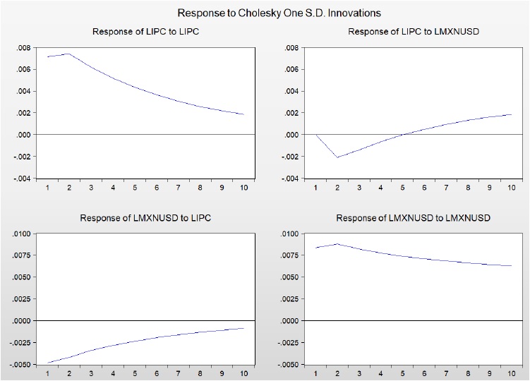
Finally, the impulse response graphical representation of the VECM models (Figure 3) shows that the response of a shock on the Mexican stock market index (LIPC) on itself vanishes away gradually, while its effect on the exchange rate (LMXUSD) first has a negative impact but five days later it is fully absorbed and, by day five, marginally enters into positive territory. In the case of a shock on the exchange rate, it initially affects the stock market negatively, and very gradually tends to disappear, after ten days. A shock on the exchange rate on itself remains present after ten days and tends to diminish very slowly.
9. Conclusion
This work presents original findings on the effects that the United States politics have on Mexican and Canadian financial markets. By analyzing the impact of public opinion polls and prediction market prices of the 2015-2016 USA presidential election on Mexican and Canadian stock markets, and on these countries’ currency exchange rates, it contributes to the literature of Efficient Market Hypothesis (EMH) and to the study of the recent USA Presidential elections influence on financial markets beyond that country’s borders.
First, the EMH states that financial markets are efficient as their prices adjust in response to any information that is relevant for the pricing of financial assets and, in this sense, arbitrage opportunities are not possible. However, surprisingly, our econometric results suggest that Canadian financial markets were not statistically affected by what happened in the American political arena.
In contrast, the information on the campaign trail was incorporated in a rapid and unbiased way on the Mexican currency and stock market. In practical terms, this regularity was helpful for portfolio managers when establishing their investment strategies. For instance, in order to beat the Mexican market, they were in a position to incorporate the anticipated effect of political news into their investment portfolios strategies, according to whether the news gave a lead to one or the other candidates. This active approach led in many cases to traders outperforming the market. Conversely, portfolio managers could take a passive approach when tracking the Canadian index.
Second, this study contributes to the debate on whether polls follow bets or vice versa. According to our econometric results using Mexican variables, polls information takes longer to be incorporated into the financial variables of interest, compared to prediction markets’ information. This finding fully agrees with the reaction time advantages that Duquette et al. (2014) mentioned in their work, but was lacking and empirical confirmation.
Third, empirical results show that country characteristics are indeed quite relevant for financial markets when affected by macroeconomic news. NAFTA was created with the purpose of having a free-trade zone to promote complementarities and impulse economic growth among its three members, Canada, Mexico and the U.S. Given the very profound differences in economic development between Mexico and the other two members, the agreement seemed quite appropriate. However, more than twenty years later the dependence of Mexico’s financial markets with respect to the political events in the U.S. proves is a fact that needs further analysis and a serious consideration from the point of view of the country’s economic development strategies. One of the stronger lessons that derive from this study’s results is the need of doing whatever it takes to reduce the Mexican economy’s dependence from a single commercial partner. Economists, think-tanks, academicians and government authorities should coordinate and develop plans and strategies to achieve that end.
Lastly, this study analyzes a quite novel topic, since there are not so many studies about the 2016 US presidential election. Empirical results reflected on the ups and downs of the campaign, plus its dramatic outcome, opened a new avenue for future research. It might be interesting to study and evaluate the impact of Trump’s policies and decisions on the other two NAFTA member countries.

