nueva página del texto (beta)
 Inglés (pdf)
 Artículo en XML
 Referencias del artículo
 Enviar artículo por email
 Citado por SciELO
  Similares en
SciELO
Similares en
SciELO 
 Permalink
1.Introduction
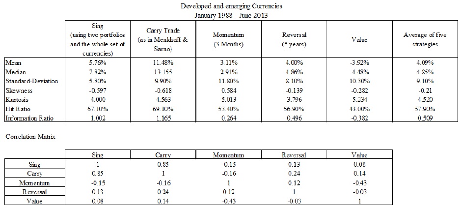
This paper studies the performance of four foreign exchange market’s common strategies that were also documented in (James, 2012). These are Carry Trade, Momentum, Reversal and Value. Among the strategies, the Carry Trade stands out; as it presents the greatest excess of returns (Castillo, 2015). Carry Trade continues to be a popular strategy, (Burnside, 2011a) proves that even if the risk of catastrophic losses is hedged using options, this kind of strategies continue to generate excess of returns. This strategy is based on the sign of the interest rate differential between a foreign currency and the US dollar. Another approach to implement the carry strategy was presented by (Lustig, 2007) and used by (Lustig, 2011) and (Menkhoff, 2011); it is based on sorting the currencies and dividing them in portfolios according to the magnitude and sign of the currency interest rate differential (Patton, 2008).
For the momentum strategy the idea is to follow the short term trend observed in the currency. The most common is using the previous returns or their average. (Barroso, 2012) suggest that there is evidence that the three months average contains information about the future behavior of the currency. (Menkhoff, 2012) shows that the predictive power of the previous return decreases when we consider returns which are further back in time or when the position is maintained for a long time. The three months period also was used by (Kroencke, 2011) while (Burnside, 2008) and (Rafferty, 2012) suggest to consider only the previous month or a twelve months lag, for which found that they contain relevant information. This approach was also applied in (Asness, 2013) without considering the most recent lag to discard the possibility of liquidity problems. Other approaches used for the momentum are based on the technical analysis. In fact, in a survey presented by (Sarno, 2002), they show that a significant number of traders follow the indicators of the Technical Analysis to take decisions about their positions in currencies.
In the case of the Reserval and Value strategies, both are based on the mean reversion property, the idea is to try to take advantage of the misalignment of the currency for its long term mean expecting a correction. These strategies were implemented in papers such as (Asness, 2013) and (Barroso, 2012) the approach changes from one reference to another. In particular (Barroso, 2012) did not obtain significant results with the Value strategies based on the real exchange rate. In our approach we reintroduce the idea of using the real exchange rate for the Value strategy to predict the returns and the deviation of the real exchange rate with respect to its long term mean. To calculate the long term tendency we use (Hodrick,1997) filter which has been used in the real equilibrium exchange rate for stochastic equilibrium models. For the reversal we use the nominal exchange rates and take as a reference the previous five years’ spot rate and using the uncovered interest parity calculate the expected value of the exchange rate taking into account the interest rate differential for the day that we want to compare to current exchange rate to determine if there is a misalignment.
The characteristics of each currency are the signals of the strategies previously constructed and it is assumed that they contain all the available information of the currency. This approach is only based on the estimation of five parameters that are assumed to be constant through time and each one is related with one characteristic and does not depend on the number of assets in the portfolio. The parsimony of the model makes it tractable to estimate the weights in which great number of assets will be invested. In the second part of the section we implement the model using the constant relative risk aversion (CRRA) utility function and a linear portfolio policy. The optimization takes into consideration the relation between the characteristic and the expected returns, and by the selection of the CRRA the optimization penalizes high volatility, negative skewness, and the excess of kurtosis. The estimated parameters only deviate from zero if they offer relevant information about the future behavior of the currency and if the combination of the parameters offers an attractive investment opportunity.
The document is divided in 7 sections, in second-one it is exposed the basics of a currency portfolio including the transaction cost, the computations of the returns and the inheritance of the positions. In the third, fourth and fifth sections each strategy is described and analyzed.
In the sixth section, we perform the parametric portfolio optimization based on the currencies’ characteristics. Finally in the seventh we present conclusions.
2.-The Foreign Exchange Market, Forwards and Currency portfolio
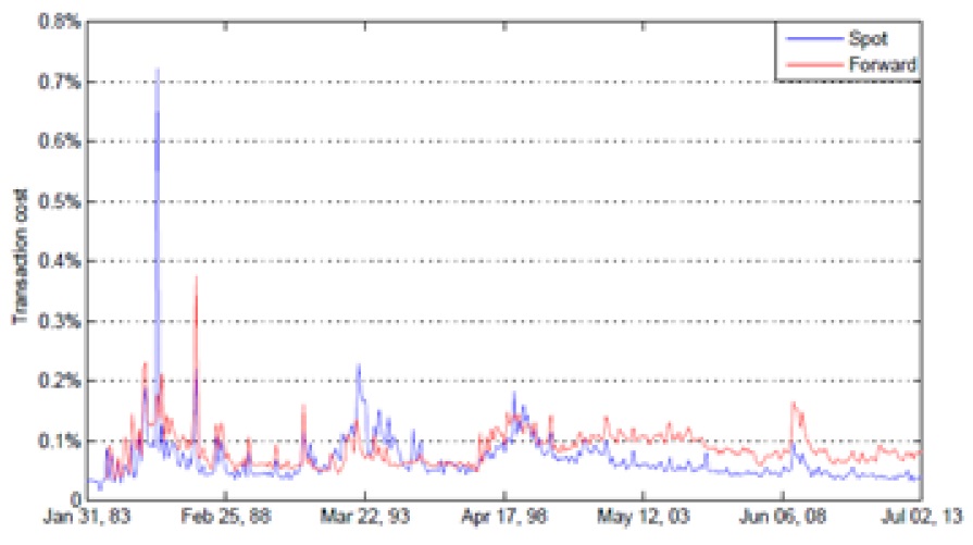
The foreign exchange market consists of all the currencies that are traded in the world, which are approximately 150. There are certain characteristics that make this market special in contrast with others, such as its decentralization, the liquidity due to the volume of trades in this market and the fact that in this market some currencies trade for 24 hours, in particular for those that are in Continuous Linked Settlement (CLS). In line with the development of the foreign exchange market the bid-ask spread has been decreasing particularly in the spot market. This has been reducing the transaction cost, which we can measure for the spot and forward prices as follows:
In the figure 1 we exhibit the average of the transaction cost for the spot and forward quotes for the 52 active currencies at each month. One of the reasons for this trend is that the foreign exchange market works with electronic media interconnected by a complex telecommunications network, including electronic trading and brokerage systems such as Reuters or EBS. These systems were complemented by the introduction of the banks’ own electronic platforms in the early 2000’s. The market share of these participants is estimated around 25% to 30% according to the BIS Market Committee (2011).
Throughout the development of the foreign exchange market, the participants have implemented different strategies, trying to obtain greater returns anticipating the currencies’ appreciations or depreciations. Among the most common is the Carry Trade, which consists of two parts, a short position in the currencies with the lowest interest rates and a long position in the currencies with the highest interest rates. Another strategy that is frequently implemented by investors is the Momentum strategy. The idea behind it is to follow the short term trend of the currency to obtain profits for the appreciation taking a long position or for the depreciation taking a short position in foreign currency. Other popular strategy is the Value, which use the long term information in order to determine if one currency is undervalued or overvalued with respect to its historical values and we propose an approach that essentially consists in buying the undervalued currencies and selling the overvalued. We use the real exchange rate which helps us determine if a currency is under or overvalued with respect to the Purchasing Power Parity (PPP).
2.1 Data for Developed and Emerging Currencies
For the purpose of this paper, the market data from the spot and forward exchange rates was obtained using the BBI (Barclays Bank) and WM/Reuters via Datastream and from the Banco de Mexico website. The Libor rate was obtained via Reuters Eikon and the Deutsche Bank Currency indexes was obtained from the Deutsche Bank’s web site dbIQ.
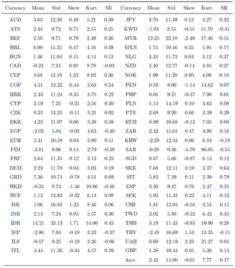
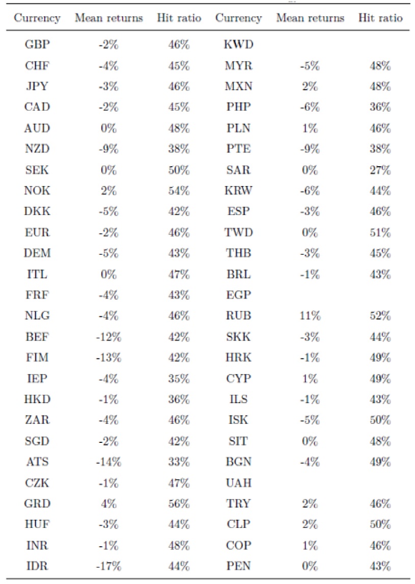
Each foreign exchange rate is expressed in number of currency units per dollar. For each one of the following 52 currencies the observed closing price in the last working day at each month was taken as a reference. These currencies are: Australian Dollar (AUD), Austrian Schilling (ATS), Belgian Franc (BEF), Brazilian Real (BRL), British Pound (GBP), Bulgarian Lev (BGN), Canadian Dollar (CAD), Chilean Peso (CLP), Colombian Peso (COP), Croatian Kuna (HRK), Cypriot Pound (CYP), Czech Koruna (CZK), Danish Krone (DKK), Deutsche Mark (DEM), Dutch Guilder (NLG), Egyptian Pound (EGP), Euro (EUR), Finnish Markka (FIM), French Franc (FRF), Greek Drachma (GRD), Hong Kong Dollar (HKD), Hungarian Forint (HUF), Iceland Krona (ISK), Indian Rupee (INR), Indonesian Rupiah (IDR), Irish Pound (IEP), Israel Shekel (ILS), Italian Lira (ITL), Japanese Yen (JPY), Kuwaiti Dinar (KWD), Malaysian Ringgit (MYR), Mexican Peso (MXN), New Zealand Dollar (NZD), Norwegian Krone (NOK), Peruvian Sol (PEN), Philippine Peso (PHP), Polish Zloty (PLN), Portuguese Escudo (PTE), Russian Ruble (RUB), Saudi Riyal (SAR), Singapore Dollar (SGD), Slovak Koruna (SKK), Slovenian Tolar (SIT), South African Rand (ZAR), South Korean Won (KRW), Spanish Peseta (ESP), Swedish Krona (SEK), Swiss Franc (CHF), Taiwan Dollar (TWD), Thai Baht (THB), Turkish Lira (TRY), and Ukrainian Hryvnia (UAH). For each one of the following 52 currencies we take the observed closing price in the last working day at each month as a reference. The set of currencies is the same that was used by Menkhoff (2011) plus the Turkish Lira, the Colombian Peso and the Peruvian Sol, other considerations for the currency selection is.
The real exchange rate index data was obtained from the BIS effective exchange rate indices using the broad and narrow indices for the currencies aforementioned with the exception of the Ukrainian Hryvnia, Egyptian Pound, and Kuwaiti Dinar whose data are not available. The indices are constructed using the geometric weighted average of the bilateral exchange rates adjusted by the corresponding relative consumer prices. The data for each month is published by the middle of the following month and the weighting pattern is time-varying, the current weights are based on trade in 2008-2010.
2.2 Currency Portfolio Description and Forward Contracts
We assume the position of a US dollar portfolio manager who wants to invest in the foreign exchange forward market and have a monthly rebalancing policy. The manager can take long and short positions in one or several currencies. To do that, the currencies are chosen every month according to the signals generated by each strategy and determine the characteristics of each currency. The value of this instrument changes during the life of the contract and has a value at maturity of
The uncovered interest rate parity (UIP) postulates that the expected foreign exchange change
(
These parities together imply the same result that we obtain from the risk neutral valuation
and as result of the estimation, should be close to zero and close to one if the market satisfies the conditions above, for instance Branson (1969). In this model we represent the new information between time and including news and economic data. Actually, there are several studies that contradict the UIP such as (Fama, 1984) who suggests that the currencies with high interest rates tend to the appreciation. For this paper the one month forward market is of particular importance; from experience we know that the most common forward contract in currencies have maturities of less than one year and in particular the tom-next, one month, and three months terms are liquid in a great number of currencies. The 2016 BIS triennial survey of FX activity confirms this, as 38.8% of the total volume in forwards has maturities less than or equal to 7 days, and 58.4% of the market share corresponds to forwards with maturities between seven days and one year; the remaining correspond to forwards with maturities bigger than one year.
2.3 Portfolio returns
The goal of this section is to introduce a framework to consider the transaction costs within the portfolio returns computation, imitating the behavior of an asset manager who tries to minimize the transaction costs by reducing the number and size of the transactions. The following approach differs from the methodologies that assume the full transaction cost such as (Lustig, 2011) considering opening and closing the whole position each month and from the (Menkhoff, 2011) approach that takes care about the inheritance in the position but does not consider the cases when only a part of the position remains in the portfolio or its amount is less than the position required for the next period. Based on the strategy to take a short or long position in the forward market, the returns obtained by these instruments in which the investor decides at inception to buy or sell in a future date a currency against USD are:
Long position return:
Short position return:
When we include the transaction cost we can rewrite the long and short positions returns for the i-th currency considering the bid and ask prices as:
Long position return:
Short position return:
Where the superscript ’a’ indicates the ask price and ’b’ the bid price for the forward and the spot. Although the transaction has been reduced in the last years, these costs have a significant impact on the returns. In practice the traders usually try to minimize this cost using the previous position as most as possible to rebalance the portfolios. When at the end of the month we have a long position in a currency that we need to renew in the forward market, the trader can synthetically replicate the forward by saving the transaction cost that comes from the sale of the long position of the i-th currency in the spot market before opening a long position in the forward market.
Under the assumption of no arbitrage we assume that the cost to replicate a long (short) position in the forward investing in the effective i-th currency (dollar) interest rate and borrowing in the effective dollar (i-th currency) interest rate is equivalent to paying the differential between the forward bid an/d forward ask prices; i.e.:
Long position return:
Short position return:
Where
Long position return:
Short position return:
where
where
When the manager has to rebalance the portfolio and may use a previous position (
Long position return:
Short position return:
When the position on the i-th currency at time
Long position return:
Short position return:
In addition, when the same position in the i-th currency has proceeded at least T-2
However this setting implies a non-continuous and non-linear problem as the
where
where
The need to use a Genetic Algorithm instead of other traditional methods of root finding comes from the function form of the
3. Currency strategies
In the following subsections we use non-parametric statistics to construct three typical strategies in the foreign exchange market without assuming any distribution. The only restriction on the currencies is that they should be active at the inception or at the rebalance date and remain active the following month and have a forward market that contains one month maturity forwards available to be traded on inception or rebalance dates.
3.1 Carry trade strategies
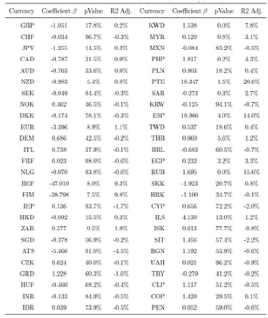
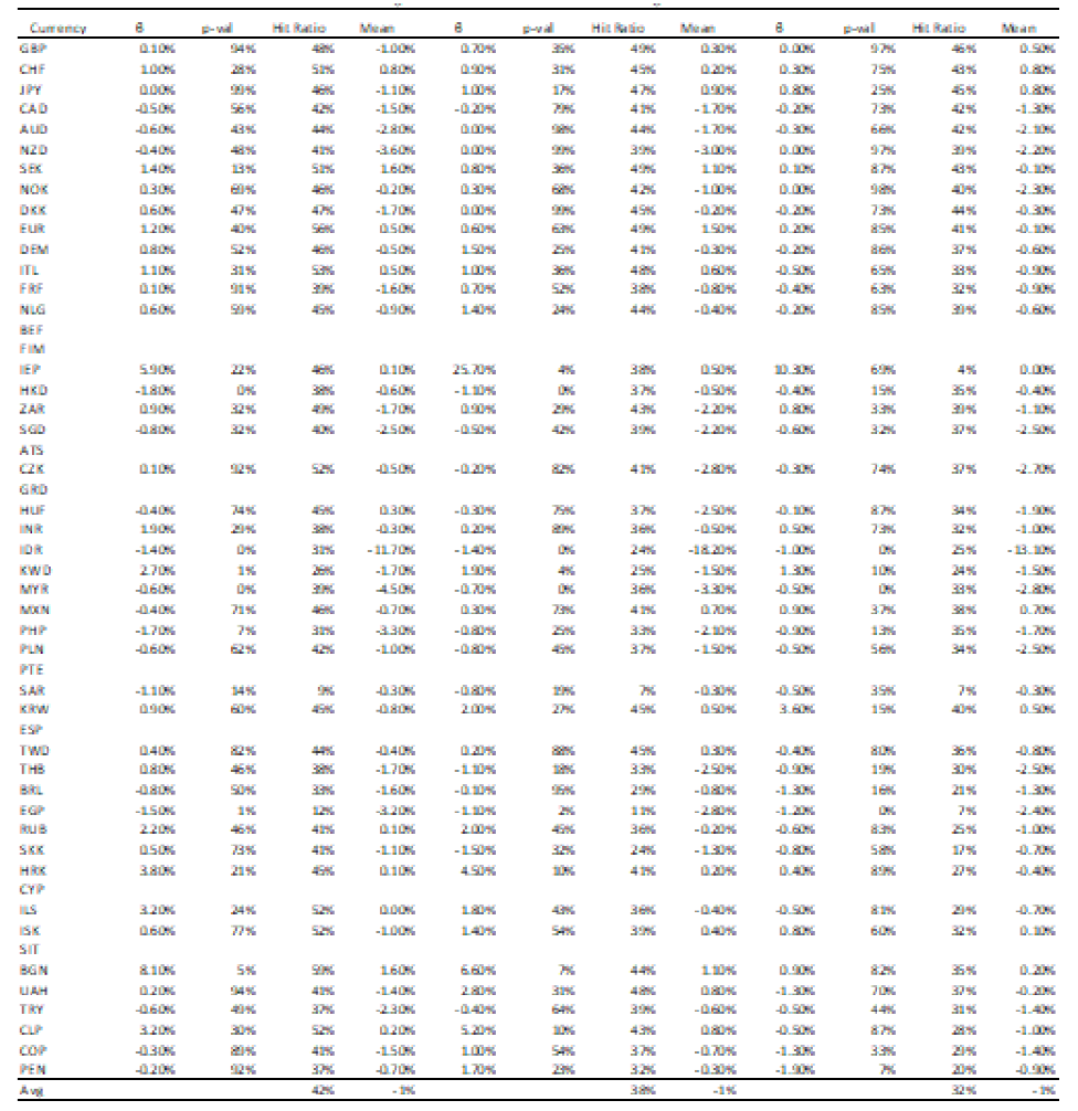
The idea behind Carry Trade is against the UIP and seeks to take advantage of the inconsistency known as the forward puzzle. Some authors have suggested that the excess of the returns generated by currencies with high interest rates is a risk compensation of unexpected events (black swans or tail events) which cause significant losses. However (Burnside, 2011a) proves that even if the risk of catastrophic losses is covered, this kind of strategies continues to generate excess returns. The table 1 shows results opposite to the UIP in its linear form, which are congruent with the results presented by Fama (1984). The intercept estimated for the regression was close to zero for all the currencies and only was significant for the KWD. Because the UIP is not fulfilled, there is a possibility to obtain positive returns from using the Carry Trade strategy.
3.1.1 Sign portfolio
The first methodology was proposed by (Burnside, 2011a) and is based on the pay-off of the carry trade:
where
This assumption allows arbitrage and implies that the UIP is not fulfilled. In order to construct a carry trade portfolio using the set of 52 currencies, we follow the next procedure: the first step consists of calculating each currency’s implied interest rate differential and sort the currencies depending on that differential, from lowest to highest. Then we separate the currencies in two sets; the first contains the currencies which have a negative interest rate differential, also called at forward discount, and the second set contains the currencies with positive interest rate differential, called at forward premium. Then with these two sets the manager can construct one long portfolio with the currencies that have positive implied interest rate differentials and a short position in the set of currencies with negative implied differentials. The strategy should be dollar neutral which means that the amount that the manager invests in the long portfolio is the amount borrowed from the short portfolio.
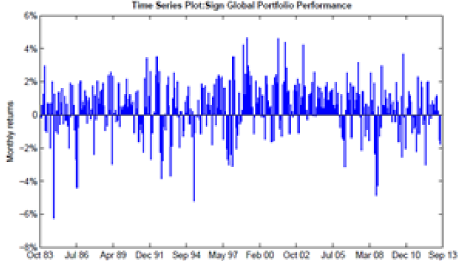
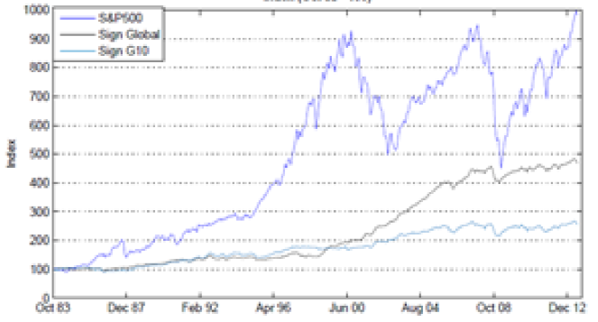
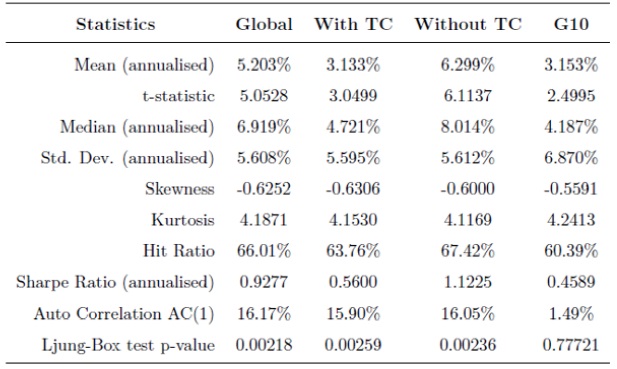
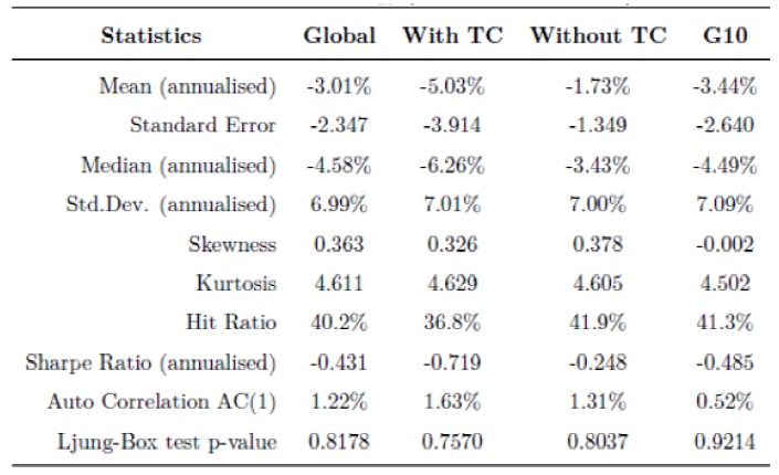
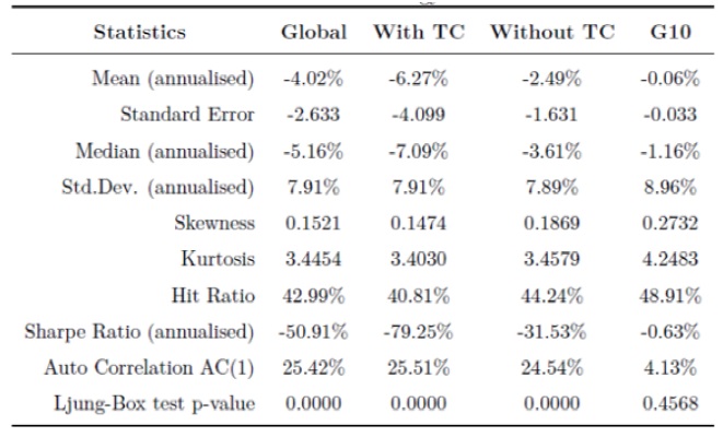
The following table shows the statistics of the Sign portfolio for the complete set of currencies that we called Global and for the portfolio that only includes the G102 currencies. Furthermore, we include the statistics of the portfolio assuming no transaction cost (TC) and another assuming that the investor pays all the transaction costs, i.e. there is no inheritance of the position in the portfolio. As a part of the statistic shown is the hit ratio which indicates the percentage that the interest rate differential (signal) forecast a positive return correctly. Finally the table includes the autocorrelation with one lag and its p-value. In the first three portfolios the auto correlation is significant, however for the G10 portfolio the autocorrelation is not significant.
3.1.2 Carry Trade High Minus Low Interest Rates Portfolio
This second approach to construct portfolios is based on the carry trade idea, sorting the available currencies at each time taking as a reference the implied interest rate differential in the forwards. The idea to sort and divide the assets into portfolios using an investment signal was originally presented by (Lustig, 2007) and was used by (Lustig, 2011) and (Menkhoff, 2011). Furthermore, the portfolios were determined by the currencies into five quantiles of 20% each.
In this case we do not know the distribution of the currencies’ im/plied interest rate differentials, then the empirical cumulative distribution function (ecf) is used to determine the quantiles and it is defined by:
where each
Each quantile determines one portfolio, in the case of the first set of currencies we assume that the manager takes a short position as this portfolio includes the currencies with lowest interest rate differentials; ideally in this portfolio there are currencies for which the differential forward-spot is negative. In the case of the other four portfolios we assume that the investor takes a long position.
Then we construct a dollar-neutral portfolio that is denoted H/L or HML following the notation of Menkhoff (2011) which takes advantage of the Carry-Trade, taking the funding by a short position in the first portfolio and then taking a long position in the fifth portfolio which contains the currencies with the highest implied interest rate differentials.
The next tables contain the statistics for the portfolios, including the cases in which there is no transaction cost, when the rebalance does not allow inheritance, and finally the portfolio constructed with the developed currencies. For the following tables, the portfolio P1 was calculated assuming a short position once we assume a long position for the other portfolios. The tables show that the transaction cost has an important effect on the mean and is less important for the other statistics. In the case of portfolio P2 the mean of returns becomes negative when the portfolio includes the transaction cost.
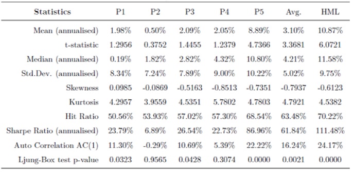
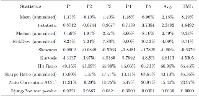
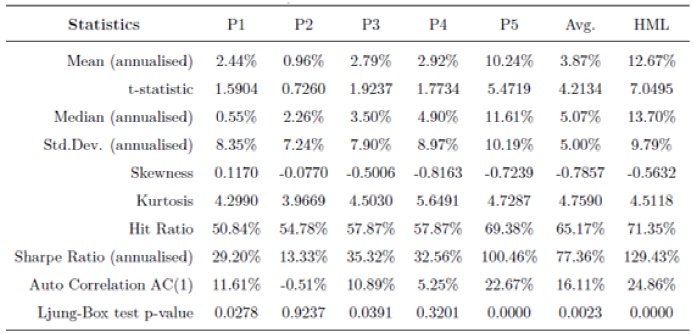
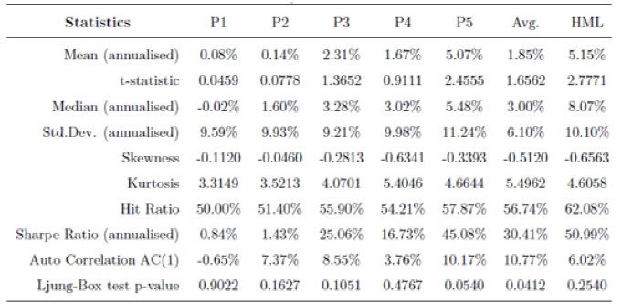
For the portfolios it is possible to appreciate that the mean increases monotonically from P1 to P5, which will be tested formally in the next section. Also we observe a rise in the levels of volatility and in the absolute value of the skewness from portfolio P2 to P5, which includes the emerging markets; in the case of the portfolios with the developed currencies the relation is not clear.

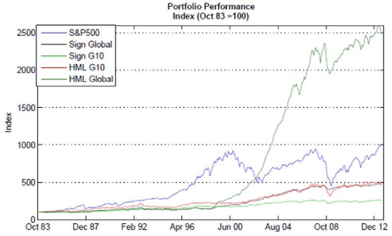
The outputs produced with the proposed method that allows inheritance do not change the statistics of the portfolios significantly, with the exception of the mean that is between the averages of the returns calculated with and without transaction costs, which was expected. In addition, the results are consistent with the results obtained by (Menkhoff, 2011) which suggest that our method, which incorporates the transaction cost in a more accurate way, is consistent with the findings in the literature. In general, the performance of the carry trade strategy for the Sign and HML portfolios is good if we compare it with S&P500, both adjusted by the level of volatility, which is lower for the carry trade portfolios. However, these portfolios showed important losses in turmoil markets as we can appreciate in the returns plots, for instance during the crisis in South Africa (1985), the crash in 1987, the crisis in Mexico (1994), the sell-off in emerging markets in 2006 and the 2008 global crisis. These observations are also made for different papers such as (Menkhoff, 2011). The losses observed in these portfolios in the crises are reflected in the negative skewness and the excess of kurtosis in the currency portfolios, particularly for those with the highest interest rate differentials. The observation of time varying risk and the Peso problem were argued by authors such as (Burnside, 2011b) and (Bhansali, 2007) as the factors that explain, to a certain point, the excesses of returns observed in the carry trade.
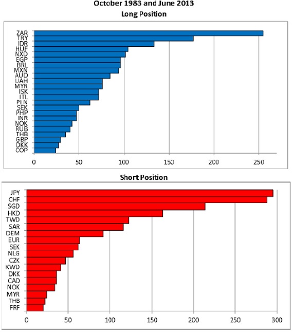
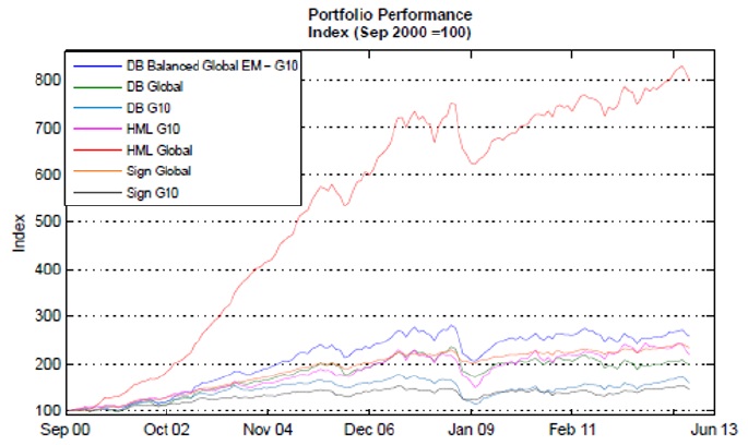
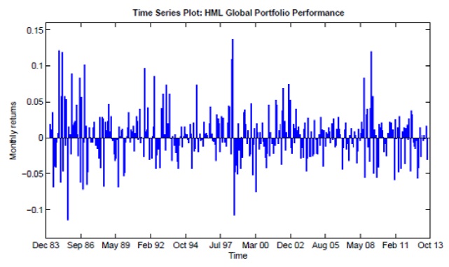
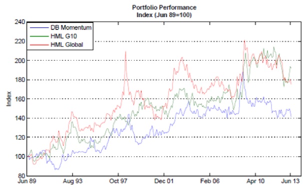
In the figure 6, the currencies that appear more frequently in the HML portfolio during the period from October 1983 to June 2013 are shown. Finally, the Sign and HML portfolios are compared with the performance of three ETF portfolios developed by Deutsche Bank3 to take advantage of the carry trade:
The DB Global Harvest Index includes the emerging and developed currencies, taking a long position in the 5 highest yielding currencies and a short position in the 5 lowest yielding currencies.
The DB Balanced Harvest Index has the same set of currencies. However it takes a long position in the 2 highest yielding G10 currencies and in the 3 remaining highest yielders from the EM, and a short position in the 2 lowest yielding G10 currencies and in the 3 remaining lowest yielders.
The DB G10 Harvest Index takes a long position in the 3 highest yielding G10 currencies and a short position in the 3 lowest yielding G10 currencies.
The HML Global portfolio that chooses the currencies from a pull of 52 showed a significantly better performance than other similar portfolios. It is also shown that the portfolios which only include developed currencies, with exception of HML G10, presented the worst performance.
3.2 Momentum strategies
The Momentum strategies are very popular in the FX markets, in particular for algorithm trading. This kind of strategies is based on the idea to buy a currency when the past performance is strong and sell the currency when the past behavior is weak. We can write the pay-off of the momentum strategy as:
where
Other periods that we find in literature, as in (Burnside, 2008) and (Rafferty, 2012), are just one month lag or twelve months, for which we found that they contain relevant information. This approach was also applied in (Asness, 2013) without considering the most recent lag to discard the possibility of liquidity problems.
The first task to construct the portfolio is to establish how many past lags in the returns we will use to determine if we should take a long or short position in the currency. In order to obtain an idea about the efficiency of this strategy, we calculate for each currency the generated returns for taking a long position when last month’s return is positive and a short position when the last month’s return is negative.
Generally, the momentum strategies that use the most recently observed returns produce profits, which is expected if we assume that the foreign exchange rate accomplishes the Markov property. Only 10 of the 52 currencies have negative returns in average, which suggests that this strategy takes advantage from the abnormalities observed in the foreign exchange market.
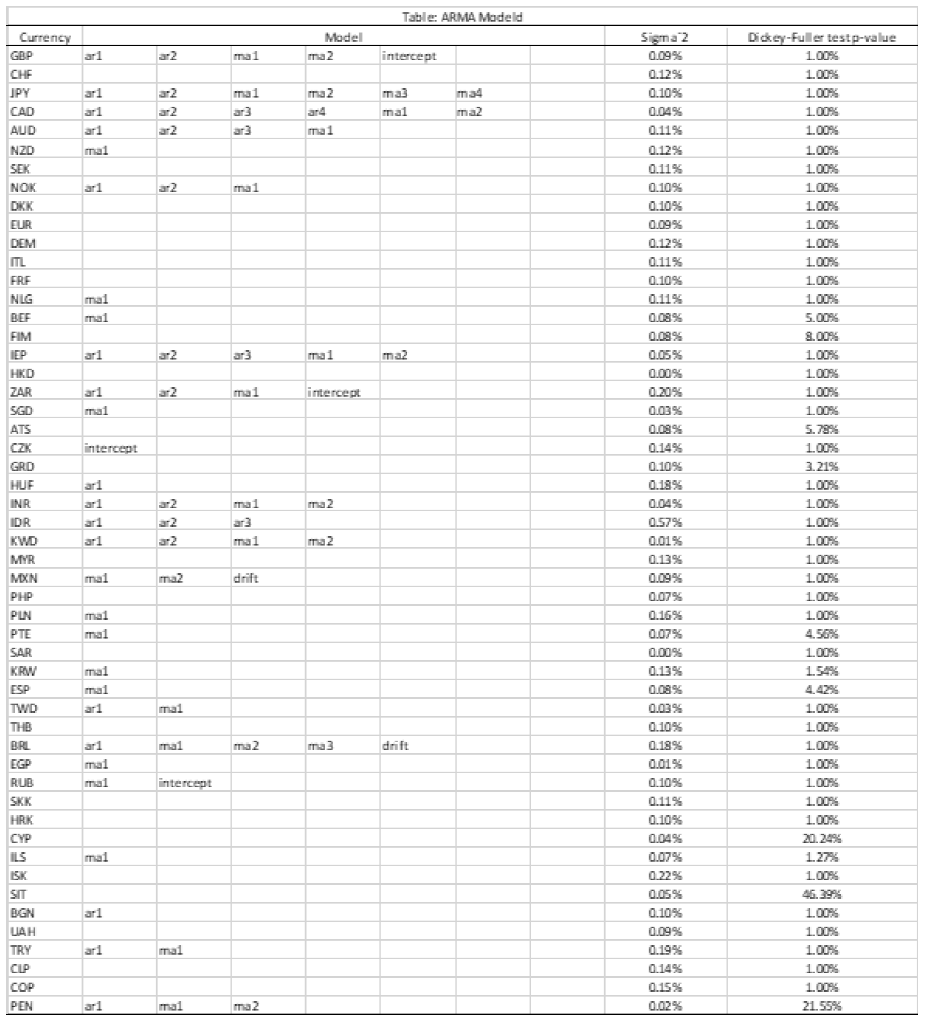
However, we analyzed if we could find significant information including more lags. In order to justify a decision in the number of lags in our average we estimate the best ARMA model based on the Akaike information criterion (see table ARMA models in the Appendix). According to the augmented Dickey -Fuller test, the majority of currencies may be stationary with p-values lower or equal to 0.0534 and the models that fit the returns in general are ARMA(p,q) with p and q lower than or equal to four. From this observation, in particular for the autoregressive part of the model, we may conclude that the number of lags should be between one and four.
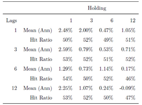
Furthermore, we compare the results with different numbers of lags and maintenance periods5 for each currency assuming all transaction costs. The following tables, which show the mean of the returns and the hit ratio of the 52 currencies using different lags and holding periods, allowing overlapping in the investments for holding periods bigger than one, suggest that the three months’ average with a holding period of one month may perform better than other combinations.
In the previous table it is possible to appreciate that the strategies that use three lags have better performance and one of the best maintenance periods is one month; for longer maintenance periods the efficiency decreases. These findings are supported by other papers such as (Menkhoff, 2012).
Following the methodology exposed in (Menkhoff, 2012) the momentum strategy sorts the available currencies in six portfolios using a cross section ranking. This method divides the pull of available currencies in 6 quantiles using the cross-sectional empirical distribution of the last three months’ returns’ average:
as it is defined above.
In order to obtain a neutral dollar strategy the first and sixth portfolios will be used to build a strategy in which the investor will take a short position in the first portfolio and a long one in the sixth portfolio (HML portfolio). It is worth mentioning that even though all foreign currencies appreciate at the same time we can take a short position in those with less significant appreciations, and long in those with greater appreciations, obtaining a benefit due to the differential between them. The analogous case is that all currencies depreciate, which allows the use of this strategy, which is dollar-neutral in any situation.
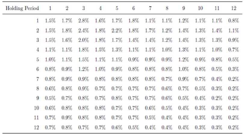

In the tables 11 and 12 we show the performance of the HML portfolios using one, three, six, and twelve months and with one, three, six, and twelve holding periods to corroborate our previous observation that three months for the average and one month holding period produces better results.
Furthermore, as with the Carry trade, we present the performance of the six portfolios and the HML portfolio. The monotonicity in the mean of return is less clear than in the carry trade and will be tested in the next chapter. Also, the results for the HML are compared with the portfolios including all transaction costs, a portfolio without transaction costs, and finally a portfolio that only includes developed currencies.


Finally, we compare the performance of the HML portfolio for the whole set of currencies and for the developed currencies (G10) with the Momentum Index6 of Deutsche Bank.
In the figure 9 it is possible to appreciate that the momentum strategy performs well during the crises, which is one of the main differences in the behavior between the momentum and the carry trade.
3.3 Value strategies
For the value strategy the principle is to determine using the real exchange rate instead if the manager will buy (sell) currencies based on under(over)-valuation relative to equilibrium exchange rates. The real foreign exchange rate considers the relative prices and is adapted according to the international commerce of each country. To show if a currency is undervalued or overvalued, we use the Hodrick-Prescott filter (HP). This filter decomposes the time series in its trend and cycle, the trend is used to determine if the real foreign exchange rate is above or below its trend line. In (Barroso, 2012) they use the standardized real exchange rate using its historical moments, they comment that this standardization is necessary as the real exchange rates are close to a unit root process. Applying the Dickey-Fuller test for the real exchange indexes, all of them reject the hypothesis to be stationary with p-values bigger than 0.01, only the NOK, the IDR, the SIT and the TRK have p-values lower than 0.05 for which the stationary hypothesis may be accepted. Furthermore, when the first differences are computed/ all the currencies accept the stationary hypothesis, then the real exchange rates are integrated once, or I(1).
In order to construct the signal, the HP filter is used to decompose the observed series
subject to
For the Hodrick-Prescott filter all the information available will be used as data for each currency. Although the returns are negative for the majority of currencies, the hit ratio is in average 45% as it is observed in the table below. The pay-off of this strategy for the i-th currency is:
where
Once again we sort the currencies from those that showed greater overvaluation to those which presented greater undervaluation using the value signal, dividing the currencies in three portfolios. Two of them are considered: The first one (PS) contains the currencies which are over its trend line and present the biggest value signal in absolute terms, and the second portfolio (PL) contains the currencies which are below its trend line and have the biggest difference. With these two portfolios the strategist should take a short position in PS and a long position in PL, building a dollar neutral portfolio. The third portfolio, PM, is also included in the tables 14 y 15.
In the following plots the performance of the value strategy is contrasted against the Deutsche Bank PPP index7


3.4 Reversal strategies
The reversal strategy is based on the idea of taking advantage of the misalignment of the currency for its long term mean expecting a correction; this phenomenon is called the mean reversion property. In this strategy the manager takes a long position in the currencies that are undervalued and a short position in the currencies that are overvalued. This strategy was implemented in papers such as (Asness et al., 2013) and (Barroso and Santa-Clara, 2012) who used real exchange rates instead of nominal exchange rates. For our purposes we use the nominal exchange rates and follow (Asness et al., 2013), who takes the previous five years’ spot rate and used the Uncovered interest parity to calculate the expected value of the exchange rate taking into account the interest rate differential (
If
In order to determine the period that we need to consider for the reversal strategy we consider three alternatives: three, four, and five years. First of all, the regression:
is calculated with the expectation to obtain a positive _ which indicates a direct relation. Although we observe that for the three-year period and for the majority of currencies the ˆ _ is positive, for most cases it is not significant. However by observing the hit ratio, this statistic indicates that in average the three years period has more accuracy anticipating the direction of the movement of the interest rate than the four-year and five-year periods.
Once we define the three-year period as a reference for this strategy, five portfolios are built by a cross sectional rank which divides the portfolios in five quantiles using the empirical cross section distribution based on the reversal signal. Then, the asset manager takes a long position in the portfolio with currencies with bigger reversal signal and a short position in the set of currencies with lower reversal. Ideally, for portfolio P5 reversal signals are positive for all the currencies and greater than the signals for other currencies. This indicates that the currencies in that portfolio should appreciate. Conversely, for portfolio P1 reversal signals are negative for all the currencies and lower than the signals for other currencies, which indicates that they should depreciate.

Only in seven months the signal is negative for all the currencies; in the other cases there is at least one currency for which it is was either positive or negative. However, if this does not happen, the strategy can also make a profit if the signal is correct, anticipating bigger returns for the currencies in P5 and lower returns for the currencies in P1.

In this strategy the losses generated for the short P1 portfolio drive the bad performance of the strategy and the monotonicity observed in the carry trade is not observed as the returns generated by a long position in P1 are bigger than the other long investments in the other portfolios in average, which contradicts the idea of the reversal strategy.
4. Currency Strategies Statistical Analysis
The goal of this section is to present a statistical analysis which includes tests of monotonicity in the carry trade and momentum portfolios, the relationships between the different strategies, and the implementation of Granger’s causality test to identify if the portfolio signals contain relevant information about the future returns of the currencies.
4.1 Non-Parametric Monotonicity and Mean tests
This section includes two subsections, both involving hypothesis tests. The first one is for the monotonicity of the returns for the trade and momentum portfolios, and the second is to test that the mean is different from zero for different portfolios of each strategy. In order to test the monotonic relations between the returns in the carry trade portfolios and in the momentum portfolios, the approach proposed by (Patton, 2008), which uses the Bootstrap methodology for the proof, will be utilized. For the sorted portfolios we have the population differences between the means of the
for
for
The idea is to reject the null hypothesis and then not rejecting the alternative hypothesis that
implies that all the
Then, using the Bootstrap we generate B new samples which were randomly drawn from the returns’sample considering replacement and considering for each sample the complete set of portfolio returns. For this paper, the size of the samples
We apply the test for the 5 carry trade portfolios assuming for this test that P1 is also a long position, and not a short position as explained in the previous chapter. Although the test does not accept the hypothesis of monotonicity with p-values above 40%, the portfolios for which this relation is not clear correspond to the portfolios for the third and fourth quintiles, i.e. P3 and P4. When the tests were made without P3 or without P4, they were accepted with p-value of 0.06 when incorporating the transaction cost and 0.03 without transaction cost. The most important relation is that the mean of returns in P1 is lower than the mean of returns in P5, which implies that taking a short position in P1 and a long position in P5 will have a positive mean of returns.
In the case of the momentum strategy, the monotonicity relation is rejected. However the monotonicity relation that the returns in P1 are lower than the returns in P6 is not rejected for the returns calculated with or without transaction costs with a p-value of 0.01. When the transaction costs are omitted, the hypothesis of monotonicity relation is rejected. This suggests that the transaction costs play an important role for this strategy. The next step is to test if the returns of the following strategies are positive in average: (1) Sign strategy; (2) HML Carry Trade strategy; (3) HML Momentum strategy, () High Value signal strategy (PL) and (5) High Value signal strategy (PL)
For the reversal and value, the High Minus Low strategy does not generate profits in average, but the portfolios with the currencies that have the higher signal showed positive returns in average. These portfolios will be used for the next test and in the next chapter to construct a portfolio that includes the five kinds of portfolios.
Let define the hypothesis:
Using the same approach as in the test before, the p-value (J) can be calculated using the bootstrap samples:
The table 19 presents a summary of these tests as well as the results from a non-parametric Wilcoxon signed rank test for the median of the portfolios’ returns. For the Wilcoxon test the hypotheses tested are:
where M is the median of each portfolio’s returns. In the table the answers presented for this test are related to

When the returns do not consider transaction costs, all the strategies reject the hypothesis that the mean is less than or equal to zero and the same applies for the median according to the Wilcoxon test. However, when the transaction costs are taken into account, only the tests for the sign and the HML Carry Trade reject the hypothesis, while in the other cases there is not enough information to reject it.
5. Granger’s Causality Test
One way to test if the signals contain valuable information to predict the future returns is through Granger’s causality test. In the standard causality test, k lags are established arbitrarily, and the following regression is performed with ordinary least squares:
with
where
The test is performed for each of the characteristics, trying to identify if these have relevant information about the future returns of the currencies. These characteristics are the following: (1) The Sign of the carry trade; (2) The Implied interest differential; (3) The Momentum signal and, () High Value signal strategy (PL) and (5) High Value signal strategy (PL) . Each one is standardized by its cross-sectional mean and standard deviation to make the series stationary. Then the Granger’s causality test is used to identify if the values in each characteristic explain the future returns of each currency.
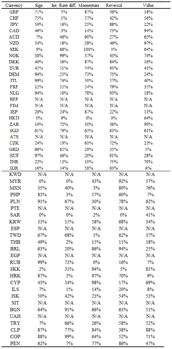
Although the results of the test show how the characteristics are relevant for some currencies and not for others, the carry trade strategies (sign and implied interest differential) are significant for a bigger number of currencies in comparison with the other three characteristics. This observation, along with the significance obtained from the mean and median tests in the last subsection, suggests that the carry trade signals contain some information that may be complemented with the other signals to construct a portfolio that takes advantage of the information contained in the four signals.
6. Construction of efficient foreign exchange portfolios
After the statistical analysis of the currency strategies in the last sections, which suggests that the characteristics of each currency contain information it is possible to construct a portfolio taking advantage of this information based on the approach of a parametric portfolio developed by (Barroso and Santa-Clara, 2012) who implement a model for a currency portfolio using characteristics for the currencies similar to those that was analyzed previously. The presented portfolios include the modification suggested by (Barroso and Santa-Clara, 2012) for the transaction costs that implicitly include information about the liquidity of each asset according to each period, which (Beardsley et al.) also incorporate in their model. Furthermore, in order to adapt the model for conservative funds such as pension funds, we propose to include a restriction in the leverage of the portfolio which may be replaced with a restriction that considers some risk budget. The efficient portfolio obtained was compared with the performance of the naive portfolio 1/N which invests in equal weights in five portfolios (Sign, HML Carry Trade, HML Momentum, P5 Reversal signal, and PL Value signal portfolios).
6.1 Portfolio optimization based on the characteristics of the currencies
For the construction of the portfolio, we use the Constant Relative Risk Aversion Utility function, also known as the power utility function. While we can apply the methodology presented in this section with other utility functions, the CRRA utility function penalizes the skewness and kurtosis as was mentioned by (Barroso and Santa-Clara, 2012) and it is explained below. The relevance of a function that takes into account higher order statistics resides in a better approximation to the investor’s preference as he or she dislikes assets with negative skewness and higher kurtosis and asks for a reward in order to accept contingency claims with these characteristics, as was mentioned by (Harvey and Siddique, 2000). For this exercise, without loss of generality, we consider:
Where
Where
In this approach the portfolio has two parts, the first one is a 100% investment in the USD interest rate and the second is a short long neutral dollar portfolio that includes
The investment in each currency is performed taking long or short positions in the one month forward foreign exchange market and the return
Another important detail about the weight function is that θT xi;t is divided by Nt, which maintains the stationarity when the number of available currencies increases or decreases, since an increment in the number of currencies may cause aggressive positions in some currencies when the implicit investment opportunities in the characteristics of the currencies are the same. For the period between October 1986 and June 2013 (the maximum period for which the five strategies were available) the minimum number of currencies was seven and the maximum was 37.
The asset manager will take a position in the USD interest rate and in the long-short portfolio when the expected utility is bigger than the utility generated by investing only in the USD interest rate:
To clarify this point, and using the Taylor’s expansion to the first order we have:
If the first order approximation is good enough, it indicates that the manager should only invest in the long short contingency portfolio if and only if it has a non-negative mean. This is a desirable condition that the optimal portfolio should fulfil. One of the advantages of using the CRRA utility function is that the investor knows its Arrow-Pratt coefficient of relative risk aversion
This optimisation takes into account the higher moments, as was mentioned earlier, and penalised the skewness and the kurtosis; this point is clearer when the utility function is substituted by its Taylor’s series around the mean:
Simplifying the notation, we can write
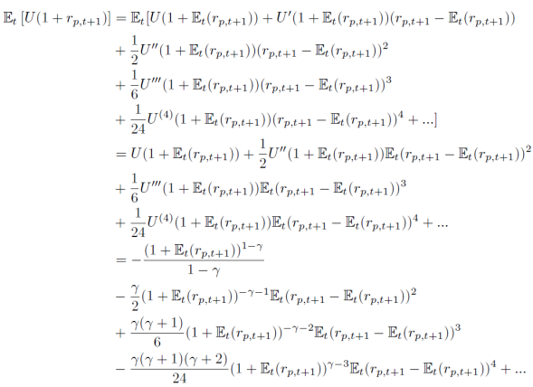
From the previous expansion it is easy to notice that for the CRRA utility function the factors in the last equation penalise the high volatility, the negative skewness, and the high kurtosis. Note that in this observation there is the assumption that
and assuming that the parameters in the vector
Furthermore, the last expression can be simplified for the non-linear optimization, using Taylor’s expansion around the mean of the portfolio returns. (van der Noll) suggest to use Taylor’s expansion of sixth order to have a good balance between the accuracy in the approximation made by the series and the computation cost to obtain the optimum.
The optimization suggested above does not take into consideration the effect of the transaction costs that also constitute a proxy of the liquidity in the market. From the analysis in the previous section it can be observed that the transaction cost and liquidity are a valid concern for the asset managers; the relevance of the transaction cost in portfolios was also reported by (Menkhoff et al.,2011) and should be treated as a separate factor from the returns. In order to incorporate the transaction cost into the optimisation, the approach of (Barroso and Santa-Clara, 2012) was followed. The modification from the previous objective function is simple, as it only needs to incorporate the forward transaction cost of each currency (
For both equations we expect that
For all
This equation can be rewritten under suitable regularity conditions as:
When the transaction cost is not taken into consideration we obtain:
If it were non-zero, then the investor could improve the utility increasing at least one of the elements which belong to
These equations are useful according to (Brandt et al., 2009) for the estimation of the standard errors using the (Hansen, 1982) approach to compute the asymptotic covariance matrix of these estimators. In the next section we calculate the standard errors using the bootstrap technique which was also suggested by (Brandt et al., 2009), in particular when the returns present leptokurtosis or when it is not desirable to make any assumption about the distribution. For the optimisation we used the following formulation in which the next constraints were included when not considering the transaction cost:
where K is the number of characteristics used for the currencies, in this setting K = 5. A similar setting is used taking into account the transaction cost in the optimisation:
The objective of restricting the values of
After the implementation of the setting proposed by (Barroso and Santa-Clara, 2012), we notice that for the currencies used in this paper the optimal parameter might generate a leverage greater than 100% of the portfolio when the leverage is measured as the sum of the weights, for which the investor takes a short position. This observation may not be a problem for the hedge funds but for market participants that take more conservative approaches such as pension funds, sovereign wealth funds, or central banks, the level of leverage necessary could limit the implementation of the optimal portfolio.With the objective of controlling the level of leverage that the implementation of the model might require and which depends on the parameters of
The idea behind the restriction is to obtain in average a leverage close to 100%. In the next section we show that the levels of leverage of the portfolio optimization are close to 100% for the computed portfolio. This restriction can also be useful in scenarios in which the short selling is restricted or when the regulation limits the short position, this limit could be over the average of leverage taken by an institution in a certain period of time. Thus the restriction contributes to the implementation of this optimization approach for a bigger number of participants.
Furthermore at the moment of solving the optimization problem, the following condition is fulfilled:
Finally and probably the most important characteristic of this approach is that it is tractable because it has a parsimonious number of parameters that have to be estimated to determine the investment amount for each currency. This fact was highlighted by (Barroso and Santa-Clara, 2012) and (Brandt et al., 2009) who avoided the dimensionality curse, that in the cases of the mean and variance optimisation and the stochastic dynamic optimisation require the estimation of
6.2 Empirical implementation and Results
In order to construct the optimal portfolios, we use the same currencies as in previous sections, and use two different windows of time. The first window corresponds to the in-sample period, which covers from October 1986 to December 1996. The second window is the out-sample period and includes from January 1997 to June 2013. The constant relative risk aversion factor that is used for the implementation is four, which was estimated empirically by (Bliss and Panigirtzoglou, 2004) using the implied information contained in the one month options for the S&P500 and FTSE. For the in-sample period, the constrained optimization of the objective that includes the transaction cost in the utility function is performed for 1,000 bootstrapped samples in order to obtain the estimation of the parameters for each sample. The same samples were used to estimate the parameters’ covariance matrix and the p-value for each parameter. Furthermore the same exercise is performed individually for each characteristic and for the objective function without transaction costs.
The samples obtained by the bootstrap allowed replacement and all of them have the same size as the original sample. The following hypothesis test is performed to determine if the estimated parameters are significant or not:
And the p-value for the parameter
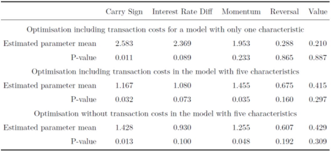

The estimated parameters for each sample are used to calculate their means, their standard errors, and their p-values. The results obtained after the bootstrap sampling and after the estimation of the parameters suggest that the momentum, reversal, and value do not characterize well the future returns of the portfolio. This is consistent with the performance and the statistics obtained for each of the portfolios, as these strategies tend to perform better than the carry trade only in stressed periods and this factor makes them valuable when they are combined with the other strategies. When the optimization is performed taking into account the five characteristics with or without considering the transaction cost inside the utility function, the significance for the momentum, reversal, value increases, and the sign and interest rate differential it decreases slightly in comparison with the high significance obtained with the model which uses only one characteristic. This is due to the sign and the interest rate differential providing similar information. (Rafferty, 2012) reported that when the strategies of Carry Trade, Momentum, and Value are combined, the asset allocation efficiency increases. This observation, along with the result of the in-sample estimation, suggests that the combination obtained using this parametric approach can outperform other portfolios such as the 1/N portfolio invested in five currency strategies or the HML carry trade alone.
For the out of sample period (OOS), the parameters

The optimal parameters change through time but in general the changes from one month to another are relatively small. In the case of the implied interest rate differential and sign strategy, the estimated parameters present an inverse relation which might be explained by the increase in the number of emerging currencies available for investments since 2000. From this year onwards, the interest rate differential has provided more information than just the sign, its magnitude has become more relevant. This is reflected in the currencies with the highest rate differentials outperforming other currencies with lower interest rate differentials even when the currencies have the same sign for the carry trade. The Brazilian Real is a good example as it has had high interest rates for a long time.
The returns obtained for the OOS period considering transaction cost and allowing the inheritance of positions clearly show more profits than losses, particularly for the period between April 2000 and December 2006. During the crisis in 2008 the portfolio presented the biggest losses and after that year the returns presented a greater number of fluctuations between the profits and losses, which may be explained by the volatile episodes in the markets observed in the last 5 years. These episodes have not been anticipated by the used characteristics of the currencies, which might suggest that a new characteristic is required to explain them. This new characteristic might be a global volatility index.
The table 29 presents the statistics of the returns obtained for the OOS period for the portfolios that were optimized with the objective function that include the transaction cost. In the first column is the portfolio that allows the inheritance of the position. The second shows the portfolio in which it is assumed that the positions are closed at the end of each period. Finally, the third column presents the results for the optimized portfolio which does not consider the transaction cost inside the objective function.
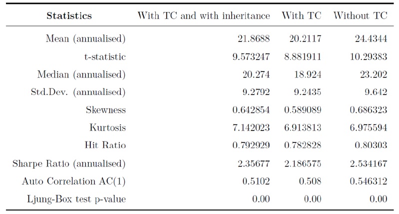
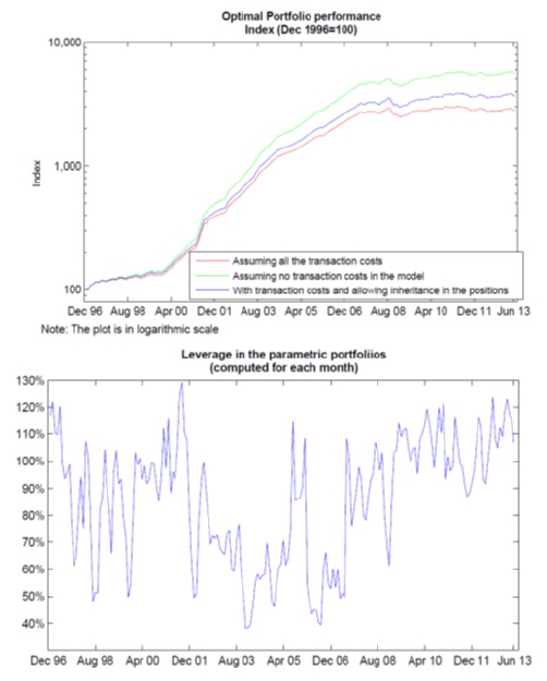
The impact of the transaction costs in the performance of the portfolio is observable in the plot as well as in the table. These costs reduce significantly the potential profits in the long run and also affect the estimations of the performance indicator such as the Sharpe ratio; for this reason the calculation is made taking into consideration the possibility to inherit the positions from one period to the next trying to replicate the behavior of an investor that tries to reduce their transaction cost in each rebalance date.
With respect to the restriction imposed in the leverage, it had a good performance preventing the portfolio from taking aggressive positions. The leverage of the portfolios OOS fluctuated between 40% and 130% which helps to reduce the crash risk of the portfolio. Additionally, the distribution of the returns of this portfolio has a positive skew and a high kurtosis, which is explained by the presence of positive returns above 10% for one month.
Another advantage of the portfolio is that it prevents taking a short position and a long position in the same currency at the same time. This might happen when an asset manager takes a position in different currency strategies. In the next few plots we compare the performance of the portfolio with the performance of the 1/N strategy that takes position in five currency strategies, with the HML carry trade, and with the DBCR+10 Deutsche Bank index.


The optimal portfolio has a much better performance than the 1/N portfolio and the Deutsche Bank index, which a similar behavior as both has diversified in analogous strategies. Even though the HML carry trade is the individual strategy with the best performance, the information contained in the characteristic produced a more profitable portfolio with less exposure to a crash risk as the estimated parameters
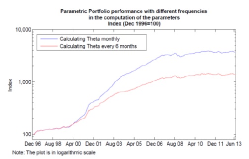
Finally, the performances of two optimal parametric portfolios were compared, the first one has the policy of re-estimating the parameters
The graph suggests that the portfolio for which the parameters
7. Conclusion
The paper formalizes and analyzes statistically four foreign exchange strategies based on the concept of carry trade, momentum, and mean reversion property. We propose a methodology to calculate the returns considering the transaction cost and allowing the inheritance of the position for the previous strategies. This method has less assumptions and incorporates the behavior of the managers who try to use their previous positions to reduce their transaction costs, which have a significant impact in the long run. Among the foreign exchange strategies, the carry trade investments (table XX) computed as in (Menkhoff, 2011), which take advantage of the interest rate differential, appear to be the most profitable against the other strategies and also contain valuable information that can be used to predict the future returns. The sign strategy that is also based on the interest rate differential show a good returns, in order of profitability the reversal and the momentum present in average profits only the value strategy in average has losses but this strategy has low correlation or even negative correlation against the other strategies that increase the diversification in risk events as this strategy tend to have a good behavior in high volatility periods. A relevant point is that the strategies returns are leptokurtic which increase the risk of big losses however a combination of this strategy that include relevant information about the future behavior of the currency decreases the risk of potential loses as the correlation among the strategies is relatively low.
In order to take advantage of the information contained in these strategies and use it to construct an optimal portfolio, we develop five signals that determine the pay-off of each strategy. These signals become the characteristics of the currencies which are used in the implementation of a version of the parametric optimization proposed by (Barroso and Santa-Clara, 2012) and (Brandt et al., 2009) to find a currency portfolio that takes advantage of the information contained in the characteristics of each currency. The adaptation of the model by the introduction of the leverage constraint produces portfolios that are more suitable to implement than the portfolios obtained without the restriction. This constraint also increases the efficiency of the sub-gradient and genetic algorithm routines applied to find the maximum.
The model also decreases the risk of in-sample over-fitting since the coefficients will only deviate from zero if the combination of them offers an increase in the expected utility.
The portfolios constructed using this method, including a constraint in the amount of leverage and taking into account the transaction cost outperform the benefits generated by the carry trade strategy or the SP500.
At least two questions remain to be investigated; the first one is to determine the optimal time for which the parameters theta should be re-estimated and if the causes of different performance is a phenomenon observed only for portfolios that include emerging currencies. The second question is if there are other signals such as the global volatility in the markets, which may contribute to the improvement of the portfolio’s performance, in particular for the last five years of the OOS sample in which there are more negative returns than in previous periods.
Finally, the performance observed in the portfolios constructed using the parametric method suggests that it could offer profitable investment opportunities that have not been used by the market participants with the exception of quant managers, who only represent a small proportion of the market participants.