


 nova página do texto(beta)
 Inglês (pdf)
 Artigo em XML
 Referências do artigo
 Enviar este artigo por email
 Citado por SciELO
  Similares em
SciELO
Similares em
SciELO 
 Permalink
JEL Classification: D31, E01, C43
"Stretching somewhat my argument about the value of data, endless billions of dollars have been spent on space exploration by the United States government just to collect a few observations of some lumps of rock and gas (with incidental kudos, 'technical spin-off' and tenuous 'defence' advantages). What government anywhere has spent one-thousandth as much in deliberately observing (experimentally or non-experimentally) or trying to understand an economic system of at least equal importance to our lives?" David F. Hendry (1980, p. 398).
"At the outset, it is worth noting that addressing the issue of rising inequality necessarily involves not just economics but also a healthy dose of political philosophy. We economists must recognize not only the limits of what we know about inequality's causes, but also the limits on the ability of our discipline to prescribe policy responses." N. Gregory Mankiw (2013, p. 22).
"The ability to replicate a study is typically the gold standard by which the reliability of scientific claims are judged." National Academy of Sciences (2002, p. 7).
1. Introduction
Tension prevails between the current statistical measurements of economic well-being and people's perception. Its consequence is obvious and inevitable: citizens are suspicious of official numbers.1 Certainly, this seriously erodes the economic and social cohesion in Mexico, among other countries. One clue to this problem is that both early and modern national accounts were designed to "provide quantitative frameworks for war-time resource mobilization and peacetime reconstruction" (Lequiller and Blades 2007, p. 398). In simpler words, accounting systems were designed to measure market production.
The gap between the government's point of view about economic performance and societal opinions is caused not only by the measurements arising in the system of national accounts, but also by other variables, markedly, the consumer price index (CPI). According to Deaton (1998,p. 43), American CPI weights are correct for households that lay at the 75th percentile of the expenditure distribution. In Spain, the applicable percentile is the 61st (Izquierdo, Ley and Ruiz-Castillo 2003, p. 149), and for Mexico, the percentile in question is the 86th (Guerrero 2010, p. 2). It is unreasonable to expect that one single plutocratic index could adequately reflect the consumption pattern of the majority in Mexico, among other countries.
As a backdrop for our analysis of the level of wealth and its distribution between families, the next figure shows household disposable income as a percentage of the Mexican economy measured by the Gross Domestic Product (GDP) between 1993 and 2012, at current prices, bases 1993 and 2008. There is no information for the first variable before the initial year.
It is worth proposing three remarks. First, changing from base 1993 to base 2008 involves a reduction of ten points of household income participation in the economy. Second, there is a slightly negative slope in the proposed measure of material well-being or, in other words, it seems that the paths of household disposable income and the economy diverge to some extent. Incidentally, Figure 1 does not address income distribution considerations. The above is an insufficiency of the measurements arising in the national account systems, which explains the following proposal made by Stiglitz, Sen and Fitoussi (2009, pp. 13-4): "Average measures of income, consumption and wealth should be accompanied by indicators that reflect their distribution. Median consumption (income, wealth) provides a better measure of what is happening to the 'typical' individual or household than average consumption (income, wealth)... It is also important to know what is happening at the bottom of the income/wealth distribution, or at the top."

Source: own calculations using data from the National Account System, INEGI.
Figure 1 Household Disposable Income as a Percentage of the Mexican Economy, 1993-2012
Third, the exercise was done using current and not constant Mexican pesos, because of the lack of information. We must remember that, in current terms, income and production are equal, but "real income" and "volume of production" are not. Assuming that price indices are correct, volume is the quantity of goods and services coming out of the "national factory door", and real income is how many goods and services (some of them produced abroad) can be purchased with the income generated in the factory. It would be desirable to evaluate the proposed ratio using constant figures. In other words, the concern about the quality of price indexes is relevant in our discussion. The heart of the matter is explained by Stiglitz, Sen, and Fitoussi (2009, p. 11) in the following quotation: "capturing quality change is a tremendous challenge, yet this is vital to measuring real income and real consumption, some of the key determinants of people's material well-being. Under-estimating quality improvements is equivalent to over-estimating the rate of inflation, and therefore to under-estimating real income. The opposite is true when quality improvements are overstated."
Our concern here refers to the measurement of economic well-being. It is clear that how well off people are, is not only a matter of income, but also a matter of wealth, in both absolute and relative terms.2 The major difficulties are that not only are financial wealth and non-financial wealth far from being correctly measured, but distributional measures are typically focused in income, and not on wealth.3
In section 1 we will review ambitious papers recently written by Davies, Sandstrom, Shorrocks and Wolff (2006 and 2010). It is remarkable that the second quoted paper was published in the prestigious The Economic Journal. No more and no less, the goal of the papers is to estimate the household wealth and its distribution for almost every country in the world in the year 2000. In doing so, the authors exercise what it is correct to call "an almost non-observed data approach". They make use of, among other resources, limited available information, regression analysis, wealth per capita and wealth distribution imputation methods, and last but not least, a large set of assumptions.
In Mexico, there are two small not compatible pieces of wealth information. The first one describes non-financial assets at a disaggregated level, basically consumer durables. The second set of data contains financial net wealth, unfortunately, at an aggregated level. Our purpose is to analyze the degree of concentration of household wealth in Mexico during its recent history. Unlike the method proposed by Davies et al. (2006 and 2010), in section 2 we will propose an observed data approach based on micro data, recorded in the open-access National Income and Expenditure Household Surveys from 1984 to 2012. To be specific, we will approximate for each sample three Gini coefficients of household wealth that will give us a broad view of wealth inequality in Mexico during intense decades of economic reforms. To our knowledge, this is an original methodology for dealing with a problem of lack of data.
Our selection of consumer durables (personal computers and vacuums), and vehicles, which apropos may constitute an income-generating assets, potentially avoids biases caused by the non-reporting and underreporting typically detected in the case of data in monetary units. In the same direction, we have eluded the huge problem linked to the determination of the values of household's wealth in the absence of observable economic transactions. While recognizing that our selection is certainly arbitrary, we note that we apply our economic intuition when selecting items that constitute a portion of household wealth.
Although our experiment is imperfect, it has the virtue of being replicable.4 In this sense, its boundaries will be revealed to the extent that in other countries, with the same lack of information, the similar empirical approximation is carried out. Attempting to put the exercise implemented here into perspective, the last section presents some final remarks.
2. Wealth Ginis: An Almost Non-Observed Data Approach
As usual, economists have more than one definition of, in our case, a household's wealth. In a broad sense, wealth is the value of all family resources, both human and non-human, over which people have command. In a more practical sense, according to a second definition, wealth is the value of physical and financial assets. In other words, wealth constitutes the family patrimony. Unfortunately, in both cases (Kennickell, 2007, pp. 3-4) "substantial technical and cognitive problems" arise, in the sense that "values of some assets, such as a personal business or a residence, may not be clear unless they are actually brought to the market; even then, there is a question of the conditions under which such a transaction might take place... Some assets and liabilities may be poorly understood, even by people who hold them."
Commonly there are two sources of information, "household balance sheets" (HBS) and "wealth surveys" (WS). According to Davies et al. (2006 and 2010) around the world only twenty two countries have "complete" financial and non-financial data, eighteen based on HBS (Canada, United States, Denmark, France, Germany, Italy, Netherlands, Portugal, Spain, United Kingdom, Australia, Taiwan, Japan, New Zealand, Singapore, Czech Republic, Poland, and South Africa), and four based on WS (Finland, China, India, and Indonesia); sixteen countries have incomplete information, among them Mexico. Using an almost non-observed data approach, Davies, Sandstrom, Shorrocks and Wolff (2006) estimated the level of wealth per capita and its distribution among households for 229 countries in the year 2000. Surprisingly, they only reported on 26 countries, leaving 12 countries with available data off of the study. Putting its strategy schematically the authors followed a two-steps process to impute both wealth levels and distribution to the countries with missing data:
1) In order to impute per capita wealth Davies et al. (2006) estimated three log-log regressions. The dependent variables were non-financial wealth, financial wealth, and liabilities, accordingly. The sample for the first one consisted of eighteen countries with HBS data and five with WS, and for the second and third regressions the sample consisted of thirty-four countries with HBS data or financial balance sheet data, and four with WS.5 Based on the existence of a strong correlation between wealth and disposable income (0.958), and wealth and consumption (0.860), the selected independent variable was the real consumption per capita. From a theoretical perspective it is difficult to argue that the relationship between income and wealth, and consumption and wealth, are linear, but for Davies et al. (2006 and 2010) it was a sufficient approximation for the empirical work.6
Using as theoretical framework a basic life-cycle model, Davies et al. (2006 and 2010) also considered five other independent variables: population density, market capitalization rate, public spending on pensions as a percentage of GDP, income Gini, and domestic credits available to the private sector. We are positive that the variables were selected at least in part due to a lack of data. In the non-financial assets regression, OLS were used, and in the financial assets and liabilities regressions the SUR estimation method was used. The authors only reported the standard errors and the "R2". It is worth mentioning that income Gini turned out to be insignificant, and goodness of fit reached almost one in each regression!
2) To estimate wealth distribution shares for countries for which no direct information existed, the authors made use of income distribution data for 145 countries recorded in the WIID dataset. Specifically, what Davies et al. (2006, pp. 23-4) carried out was the following:
"The common template applied to the wealth and income distributions allows Lorenz curve comparisons to be made for each of the 20 reference countries... In every instance, wealth shares are lower than income shares at each point of the Lorenz curve: in other words, wealth is unambiguously more unequally distributed than income. Furthermore, the ratios of wealth shares to income shares at various percentile points appear to be fairly stable across countries, supporting the view that income inequality provides a good proxy for wealth inequality when wealth distribution data are not available. Thus, as a first approximation, it seems reasonable to assume that the ratio of the Lorenz ordinates for wealth compared to income are constant across countries, and that these constant ratios (14 in total) correspond to the average value recorded for the 20 reference countries. This enabled us to derive estimates of wealth distribution for 124 countries to add to the 20 original countries on which we have direct evidence of wealth inequality."
Davies et al. (2006 and 2010) did not provide any assessment about the validity of their results, specifically speaking about their imputation methods that essentially generated the Gini coefficients for the basket of countries included in the analysis. Being in their shoes, one way would have been to take, as a control mechanism, a country with available information. On the point, Davies et al. (2008, pp. 30-1) mentioned the following:
"Other respects also lead us to believe that our estimates of the top wealth shares are conservative. The survey data on which most of our estimates are based under-represent the rich and do not reflect the holdings of the super-rich. Although the SCF (Survey of Consumer Finances) survey in the USA does an excellent job in the upper tail, its sampling frame explicitly omits the 'Forbes 400' wealthiest US families. Surveys in other countries do not formally exclude the very rich, but it is rare for them to be captured. This means that our estimated shares of the top 1 per cent and 10 per cent are likely to err on the low side. A rough idea of the possible size of the error can be gained by noting that the total wealth of the world's billionaires reported by Forbes for the year 2000, $2.16 trillion, was 1.7 per cent of the total world household wealth we find here, of $125.3 trillion."
A relative insufficiency of Davies et al. (2006 and 2010) is linked with the fact that the "statistical adequacy" of the regressions was not tested, that is to say, their model is not transferable (Granger, 1993, p. 3)7. We would say as a corollary that its exercise is not replicable.
Davies et al. (2006, p. 26) concluded the following: "our wealth Gini estimates for individual countries range from a low of 0.547 for Japan, to the high values reported for the USA (0.801) and Switzerland (0.803), and the highest values of all in Zimbabwe (0.845) and Namibia (0.846). The global wealth Gini is higher still at 0.892. This roughly corresponds to the Gini value that would be recorded in a 10-person population if one person had $1000 and the remaining 9 people each had $1."8
3. Wealth Ginis: An Observed-Data Approach
The National Income and Expenditure Household Surveys (ENIGH) compiled by the INEGI, the Mexican national statistical institute, include information about some durables goods, among others, the number of personal computers (PCs),vacuums and vehicles owned by each family. The surveys do not distinguish between laptops and desktops, so the records include both types. Somewhat the same applies for the vacuums. The wealth variable "vehicles" includes three types: cars, vans, and pick-ups. The following tables contain information about the number of PCs, vacuums and vehicles as percentages of the total families. Please note that the information is presented in physical units, which may constitute an advantage to the extent it avoids well-recognized biases detected in monetary data. In addition, using physical units we do not have to rely in the values of used vehicles determined by households in the absence of "observable economic transactions".
Table 1 Number of PCs as a Percentage of Total Households
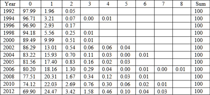
Source: own calculations using data from ENIGHs.
Over the years, there is a decrease in the percentage of families that do not have a PC, going from 97.99 percent in 1992 to 69.90 percent in 2012. In other words, there is a significant increase in the percentage of households that have at least one PC, from 1.96 percent in 1992 to 24.47 percent in 2012, which means an increase of nearly twenty-one points within the period under review. On the other hand, according to the OECD Mexico ranks last in households with access to a computer at home. Chile, the second worst ranked, doubles the Mexican IT penetration.
The case of vacuums is moderately different from that of PCs and from that of vehicles, as we will see in a moment. Basically, it displays a fairly rigid behavior throughout the analyzed period. Stated otherwise, as time goes by as a constant less than ten percent of households own a vacuum. The content of the Table 2 are core data extracted from the surveys. This information not only reveals the lack of access to a durable good, but also shows the "pre-modern style" in the cleaning process in the Mexican home, which evidently can be analyzed from a gender perspective.
Table 2 Number of Vacuums as a Percentage of Total Households

Source: own calculations using data from ENIGHs.
Table 3 Number of Vehicles as a Percentage of Total Households

Source: own calculations using data from ENIGHs.
In 1984, the vast majority of families did not own a vehicle. However, in 2012 almost one third of households in Mexico owned at least one vehicle. It is also clear that, as time goes by, the number of families that may have access to a greater number of vehicles has also slightly increased. Unfortunately, the surveys do not register if the vehicle is used simply as transportation by the family, as a taxi, that is, as an income-generating asset, or as collection purpose.
Numbers are difficult to internalize, so to get the message inside our heads the following figure shows Gini coefficients for PCs, vacuums and vehicles that may be estimated based on the ENIGHs, the wealth Gini reported by Davies et al. (2006), and the official income Gini for Mexico between 1984 and 2012.9 On one hand, considering that we are not taking into account the value of the selected items, the proposed Gini coefficients are probably optimistic.10 On the other, the lack of monetary data constitutes a source of bias in our measures.
Figure 2 is fascinating, and invites speculation. Suffice to say the following. It is a welcomed statistical coincidence that, in 2000, wealth Gini figure estimated by Davies et al. (2006) and the one derived from the vehicles proposed here are almost equal. Agreeably a third study, written by Torche and Spilerman (2008), obtained a similar value. To be specific, using home ownership distribution for the year 2000 the mentioned authors estimated wealth Gini coefficients for some Latin American countries. For Mexico, the figure reported was 0.70.11

Our observed-data approach allows us to garner information about the trend of the wealth Gini coefficients in Mexico between 1984 and 2012. In this regard, it should be noted that this document offers the first available time series of Mexico's wealth Ginis, nonexistent for many economies, advanced and emerging. Figure 2 shows that, although the patterns of wealth and income Gini coefficients are somewhat different, under the current development strategy the distribution of both are downwardly rigid. Thus, after decades and decades of aggressive economic reforms the distribution of well-being remains vastly unequal. Based on our comprehension of the Mexican reality, we are led to propound that the inefficiencies of markets and government and market failures in a broad sense are the underlying causes of this kind of uneven distribution. And we suspect most people would agree.
Frequently the literature does not give emphasis to the feedbacks between macroeconomic performance of countries and its wealth distribution patterns. For example, in their comprehensive study on the determinants of economic growth, Durlauf, Johnson and Temple (2005) found approximately as many explanatory variables as there are countries for which data are available. To be specific, they listed 145 different regressors statistically significant, which reveals, among others concerns, a data mining generalized practice in the applied economic analysis. It is shocking that only five papers in their review included the income distribution as an explanatory variable, and that two of them argued a positive effect and three a negative one. Only in the paper written by Alesina and Rodrik (1994) the wealth distribution was proposed as a determinant of economic growth. Unfortunately, their perspective was merely theoretical because of a lack of data. Here we want to highlight the following consequences of the extremely unequal wealth distribution in Mexico. An obvious one is the deterioration of economic and social cohesion.12 The social capital, which is a genuine accelerator of the well-being in the modern societies, has not been sufficiently accumulated along the analyzed period in Mexico, partially explaining its disappointing performance vis-à-vis other countries that have implemented similar economic reforms.
According to the literature, the material well-being is related to income, consumption, a dimension not considered here, and wealth. Here we analyzed income and wealth distributions separately, but a joint perspective would imply another inequality, that is to say, "the inequality of achievement across dimensions for the same individual" (Ruiz, 2011, p. 16; see also Jantii et al. 2008). To get an intuitive understanding of this second inequality, Ruiz (2011, p. 16) wrote the following example: "units achieving a relatively lower level of wealth in comparison to income and consumption are at greater risk of experiencing future economic hardship, facing low-consumption possibilities in the future if their income drops. Their material conditions could thus be seen as worse than having a bit less income but higher wealth."
In order to close this section we work out an illustration about the meaning of a Gini coefficient equal to 0.667, that is the vehicles Gini obtained for the year 2012. Our assumptions are the following. The first decil has a wealth equal to one Mexican peso. In order to determine the wealth from the second to the fifth deciles we applied the same observed ratio between the decil in question with respect to the first decil considering its "current monetary income" registered in the ENIGH 2012. This is because it is not until the sixth decil that households are in an economic position to save. In order to determine the wealth from the sixth to the tenth deciles we just applied a constant integer.
Based on ENIGH 2012 it is correct to say that the "current monetary income" observed ratio between the last and the first deciles was 19.0, and the two top deciles owned 50.9 percent of the "current monetary income". The income Gini coefficient reported in the same year was 0.440. In our wealth simulation, the ratio was 98.9, and the two tops deciles owned 72.5 percent of household wealth.13
Our simulation is consistent with the perspective advanced by Kennickell (2007, p. 6), who compared income and wealth distributions using observed data for the US: "The levels of income and wealth are quite different across their distributions... Income is higher than wealth at the bottom of the distribution and substantially lower at the top... Comparison of the quantiles of each distribution shows that the distributions also differ greatly in relative terms, with wealth being proportionally far higher in the upper tail of the distribution."
4. Final remarks
It seems that the study of the distribution and composition of household financial and non-financial wealth is currently a flourishing research field. However, this literature faces serious difficulties. For example, according to Jantti, Sierminska and Smeeding (2008, p. 5), "household surveys of assets and debts, for instance, typically suffer from large sampling errors due to the high skewness of the wealth distribution as well as from serious non-sampling errors. In comparative analysis, these problems are compounded by great differences in the methods and definitions used in various countries. Indeed, in introducing a collection of essays on household portfolios in five countries, Guiso, Haliassos and Jappelli (2002, pp. 6-7) mention 'definitions' as the 'initial problem' and warn the reader that 'the special features and problems of each survey ... should be kept in mind when trying to compare data across countries'."As a result, even a project such as the Luxemburg Wealth Study has been able to analyze wealth distribution exclusively in five countries. In this sense, the papers written by Davies, Sandstrom, Shorrocks and Wolff (2006 and 2010) are seminal.
Unlike the almost non-observed data approach designed by Davies et al. (2006 and 2010), in order to estimate household wealth Gini coefficients from 1984 to 2012 we proposed an observed data approach, which represented the intensive utilization of 14 open-access surveys. This paper's main contribution resides in a display of a historical view of wealth distribution during a period of intense economic reforms in Mexico, among other countries.
To provide an assessment about the validity of their results, both Davies et al. (2006 and 2010), and Torche and Spilerman (2008), applied a second best solution. The above is explained by the empirical nature of the investigated problem. Unfortunately, in our case the other wealth information available in Mexico is merely in levels and covers just a few recent years, so it is not suitable for our purpose nor is it useful to provide any assessment about our results. Hence, we rely on the fact that the statistical values obtained by Davies et al. (2006 and 2010), and Torche and Spilerman (2008), and the ones obtained here are similar. Considering that we did not take into account the value of the selected items, the proposed Gini coefficients are probably downward biased.
Looking to the bright side of our imperfect approach, we want to emphasize that our selection of assets potentially avoids biases caused by the non-reporting and underreporting typically detected in the case of data in monetary units. In the same direction, we have eluded a huge problem linked to the determination of the values of household's wealth in the absence of observable economic transactions. Last but not least, our approach has the virtue of being replicable, a scientific tool that should be used much more in economics.
To close it is indispensable to introduce another relevant perspective, which comes from the political economy of measurement in economics. As stated by Hulten (2004, p. 10), "like all other aspects of government in a democratic system, a nation's statistics are ultimately subject to the consent of the governed." It suffices to say that, statistically speaking, we live in an almost perfectly unequal world, of which Mexico is a clear example. Without doubt, the above constitutes valuable information that potentially may displease many citizens in Mexico and worldwide.


