


 nova página do texto(beta)
 Inglês (pdf)
 Artigo em XML
 Referências do artigo
 Enviar este artigo por email
 Citado por SciELO
  Similares em
SciELO
Similares em
SciELO 
 Permalink
1 Introducción
Anaerobic digestion (AD) has recently gained considerable importance as a waste treatment technology to reduce organic matter in agro-food industries and municipal effluents. The AD process presents advantages compared to aerobic treatment as: short hydraulic retention times, low sludge production, high organic load removal, and low initial and operating cost. Recently, much attention has been paid to AD of the organic fraction of municipal solid waste (OFMSW) as an attractive option technology for efficient treatment and simultaneous production of a renewable energy source through the use of biogas (Mata-Alvarez et al., 2000). Nevertheless, its widespread application has been limited, because of the complexity of the process, and difficulties involved in achieving a desirable operation of the AD process. All these aspects can be overcome with the development and improvement of instrumentation and control systems (Jimenez et al., 2015; Méndez- Acosta et al., 2008). Moreover, with a suitable dynamic model it is possible to evaluate the AD process behavior and to formulate and evaluate control strategies. These models are also used in the modeling, identification, design, optimization, and on-line monitoring of AD process (Gómez-Acata et al., 2015; Cuevas-Ortiz et al., 2015).
The availability of a simple AD model is desired as it captures the complexity of the process, and allowing the sustained operation under a feedback control law. Because of this, many studies have been devoted to this aim. Kiely et al. (1997) proposed a nonlinear dynamical model of AD of OFMSW based on three previous models (Hill and Barth, 1977; Moletta et al., 1986; Havlik et al., 1986). The model includes: hydrolysis, acidogenic and methanogenic processes, the growth kinetics of acidogenic and methanogenic bacteria; also considered equilibrium between CO 2 and HCO −, cations and NH +4; finally inhibition by ammonia in the growth kinetics of methanogenic bacteria were also considered. Esposito et al. (2008) described the dynamical anaerobic co- digestion processes of OFMSW and sewage sludge. The model (Esposito et al., 2008) describes the surface based kinetic behavior of the OFMSW disintegration process. From this seminal idea several studies have been reported which include model calibration and validation (Esposito et al., 2011a), effect of the organic loading rate (Esposito et al., 2011b) and enhanced bio-methane production from co-digestion. Other contributions are based on distributed parameters. In this sense, Vavilin et al. (2003) and Nopharatana et al. (2003) take into account the change of a set of parameters in the mathematical model involving the flow liquid inside of the digester. Kinetic modeling have been also reported for batch process of AD of MSW (Nopharatana et al., 2007) and semicontinuous OFMSW (Fernandez et al., 2010) under specific operational conditions. Pavan et al. (2000) reported the kinetic study of a two-phase AD process using diffusional models; in addition, a comparison with a single phase system is also carried out.
A theoretical principle states that the set of operational conditions for AD process allows one to set operational condition and, after that, to propose feedback schemes to control and preserve such operational conditions. Nevertheless, in order to predict how the system responds during or after a change of operational conditions is convenient a mathematical model. The analysis of the dynamical model allows us to formulate changes of operational conditions and control strategies for the AD process (Nopharatana et al., 2003). Although, Alatiqi et al. (1994) analyzed AD mesophilic and thermophilic processes schemes in terms of stability and controllability, it is not clear yet the role of the inhibition phenomenon. In same direction, Bolzonella et al., (2003) studied the variations of the process parameters during transient conditions and identified dynamical behavior between changes of stable conditions and parameter behavior; nevertheless, there are not predictions of key variables under an inhibition scenario.
Although several mathematical models reported describe the AD process of organic solid phase (Kiely et al., 1997; Esposito et al., 2008; Fernandez et al., 2010), a model is desirable such that operational conditions can be captured and control strategies can be formulated in face to diverse scenarios. Because of operational stability of the AD process is largely dependent on the accumulation of VFA, a model should include the dynamical behavior of VFA inhibitory phenomenon. To our knowledge, only a few contributions, among those that have addressed the VFA accumulation, have identified acidification as open-loop stable operational condition (Méndez- Acosta et al., 2008; Myint et al., 2007). Moreover, the problem of the operational instability due to the accumulation of VFA remains open. In this study a mathematical modelling of AD process and mathematical analysis is addressed towards control design. The first objective is the design a mathematical model as simple as possible in terms of main key variables. The technical difficulty resides in the capability of the model to captures the dynamics of the main operation conditions of real continuous AD process as washout condition, acidification condition and normal operation condition. The second objective is the design a control scheme that is capable of regulating the VFA concentration in continuous AD process.
This contribution is organized as follows. A reduced dynamical model is proposed and dynamic features are exposed and analyzed in Section 2. In Section 3, a control problem is formulated for a continuous AD of OFMSW process. Then, in Section 4, a PI classical feedback controller is derived and some simulations are shown in order to illustrate the performance of the controller. Finally, some concluding remarks are addressed.
2 Model description
The dynamical model is derived from previous proposals (Hill and Barth, 1977; Moletta et al., 1986; Kiely et al., 1997). The model describes the dynamical behavior of AD process of OFMSW through a set of nonlinear ordinary differential equation (ODE). Each ODE is based on mass balance of components of the continuous isothermal AD process. For overall AD for OFMSW includes four steps: hydrolysis, acidogenesis, acetogenesis and methanogenesis. The hydrolysis is recognized as the rate-limiting step for overall AD process, while methanogenesis is the rate-limiting step for easily biodegradable substrates (Ariunbaatar et al., 2014; Fernández-Gu ̈elfo et al., 2011). The separation of the hydrolytic stage from the methanogenic enhances a stable development of each biochemical reaction, promoting organic matter degradation and biogas production. Pretreatment for the organic solid fraction and OFMSW might be needed in order to ensure the transformation of insoluble organics matter to soluble compounds (Ariunbaatar et al., 2014; Cesaro et al., 2014). Thus, the hydrolysis stage is neglected in the model but assumed to be performed at previous pretreatment stage.
The relation among microorganisms and substrates is defined by mass balances under isothermal condition. Four substrates are considering: soluble organic mater, volatile fatty acids, ammonia and methane. Acidogenic and methanogenic bacteria are included in the model. The inhibition by volatile fatty acids has been considered into the specific grow rate of acidogenic bacteria. In addition, ammonia and volatile fatty acids inhibition are included into the specific grow rate of methanogenic bacteria. The processes start with the degradation of organic soluble matter. Continuous production of soluble organic matter is supposed by the enzymatic action of the acidogenic bacteria. In the next stage, acidogenic bacteria produces a series of acids. Nevertheless, only acetic acid is considered in the model. Finally, acetoclastic methanogenic bacteria converts acetic acid to methane. The pH is assumed constant and the ionic dilute equilibrium is preserved. The pressure is assumed constant P = Patm ; which means that despite of the fact that there is a continuous production of mixture of gases (CH 4, CO 2, NH 3) the pressure of the AD process is maintained to Patm . Then, the produced mixture of gases is assumed to go directly out of the digester. The NH 3 production rate is supposed less than methane and carbon dioxide rates. During biochemical reactions CO 2 is also produced. Nevertheless, as operating conditions (pH, temperature and pressure) and ionic equilibrium are preserved, the relation between CH 4 and CO 2 is assumed constant. Then, CO 2 and NH 3 gas production rate are not modeled. Under above assumptions and conditions, the dynamical behavior for acidogenic biomass is described by (Hill and Barth, 1977; Moletta et al., 1986):
 (1)
(1)
where X 1 is the acidogenic biomass [mg/l]; KD1 is related to the death rate of acidogenic biomass [d −1]; D is the dilution rate [d −1]; and μ 1 is the specific growth rate of acidogenic biomass [d −1] defined by (Kiely et al., 1997):
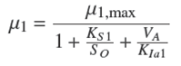 (2)
(2)
where μ1,max stands for the maximum specific growth rates [d −1]; KS1 denotes the saturation constant for the acidogenic bacteria growth [mg/l]; KIa1 is the inhibition constant of acidogenic bacteria growth [mg/l] which is related to volatile acid inhibition; S O is the soluble organic matter concentration [mg/l]; and VA is the volatile acid concentration [mg/l]. The dilution rate D [d −1] is defined as the ratio of the inlet flow rate Qin [ld −1] respect to the reactor volume V [l]. The dynamic description for methanogenic biomass is described by (Hill and Barth, 1977; Moletta et al., 1986):
 (3)
(3)
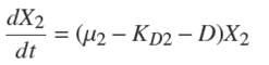
where X 2 is the methanogenic biomass [mg/l]; KD2 is related to the death rate of methanogenic biomass [d −1]; D is the dilution rate [d −1]; and μ 2 is the specific growth rate of methanogenic biomass [d −1] defined by (Kiely et al., 1997):
 (4)
(4)
where μ 2,max is the maximum specific growth rates [d −1]; KS2 is the saturation constant for the methanogenic bacteria growth [mg/l]; KIm1 is the inhibition constant of methanogenic bacteria growth [mg/l] which is related to volatile acid inhibition; KIm2 is the inhibition constant of methanogenic bacteria growth [mg/l] which is related to inhibition by ammonia. The mass balance of the first stage is the dynamic of soluble organics S O [mg/l] consists of the following terms: (i) inlet-outlet mass balance related with dilution rate D; (ii) consumption by acidogenic bacteria with a yield coefficient YX1 [mg X 1/mg SO ]; and (iii) production by acidogenic bacteria with a yield coefficient YX1SO [mg X 1/mg SO ] (Hill and Barth, 1977).
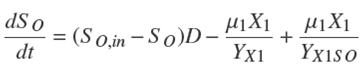 (5)
(5)
The mass balance of the volatile organic acids VA [mg/l] consists of the following terms: (i) inlet- outlet mass balance related to the dilution rate D; (ii) production by acidogenic bacteria with a yield coefficient YX1VA [mg X 1/mg VA ]; and (iii) consumption by methanogenic bacteria with a yield coefficient YX2VA [mg X 2/mg VA ] (Hill and Barth, 1977).
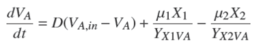 (6)
(6)
The mass balance of NH4 [mg/l] consists of: (i) inlet- outlet mass balance related to the dilution rate D; and (ii) production by acidogenic bacteria with a yield coefficient YNH4 [mg X 1/mg NH 4] (Kiely et al., 1997).
 (7)
(7)
As low pressure operation and diluted system condition is assumed, mass transference of NH 3 between liquid and gaseous phases is neglected. Then, the term related to gas-liquid mass transference of ammonia is not included in equation (7) (Kiely et al., 1997).
Because of both ionic equilibrium and pH constant value are assumed, a linear relation between NH 3 and NH 4 is defined by:
 (8)
(8)
where NH 3 is the concentration of ammonia [mg/l]; NH 4 is the concentration of ammonium [mg/l]; KNH4 is a constant which consist of the following parameters: KiNH4 = 5.3 * 10−10 @ 35 ◦C the ionization constant; [H+] is the hydrogen ion concentration (pH = −log[H +]); and the mol weight of NH 3 and NH 4 stand for MNH3 and MNH4 respectively. For the proposes of this work the pH is considered constant (pH = 7.0).
The methane gas flow [(lCH4 /lreactor )d −1] is described by the following algebraical equation (Kiely et al., 1997):
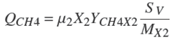 (9)
(9)
where YCH4X2 is the yield coefficient for methane forming bacteria [mol CH4/mol org]; SV = 25.4[l/mol @ 35 ◦C] is the standard volume; and MX2 = 111300[mg org/mol org] is the mole weight of organisms (Hill and Barth, 1977). Under temperature and pressure operating conditions there is very low solubility of methane in the liquid phase. Therefore, methane in liquid phase is neglected. Then, the AD model is defined by a set of differential equations:
 (10)
(10)
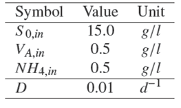
which describes the dynamical behavior of AD process for OFMSW, where the states variables stand forΦ=[X 1,X 2,SO ,VA ,NH 4]andanalgebraicrelation of CH 4 production. The set of parameter π = {μ 1max, μ 2max, KD1, KD2, YX1, YX1SO, YX1VA, YX2VA, YNH4, KS 1, KS 2, KIa1, KIm1, KIm2, KNH4 } are real and uncertain constants. The nominal values π0 ϵ π and additional parameters are shown in Table 1.
Table 1 Specifications for parameters. HB means obtained from Hill and Barth, (1977); and K from Kiely et al. (1997). Notice that KNH4 comprises several parameters (see (8))

Departing from AD model (10) a complementary analysis is desirable to determine which parameters in π affect the dynamical behavior of the field ƒ (Φ, π). Then, to address the behavior of ƒ (Φ, π) if the parameter values have changed, a sensitivity parametric analysis (Khalil, 2002) has to be done. For a set of parameters π, the approximate solution for the sensitivity function S ƒ (t) = Φπ (t, π0) is computed by the simultaneous solution of the nonlinear nominal AD model (10) and the linear time-varying sensitivity equation (Khalil, 2002):
 (11)
(11)
where S ƒ ϵ R 5×15. The Fig. 1 shows the solution of equation (11) respecting to parameter set π (Table 1), nominal operating condition (Table 2) and initial condition Φ0 = [1, 1, 1, 1, 1] T . The parameters subset having the most significant effect on dynamical behavior of AD model (10) are μ 1max ,μ 2max ,KD1 , KD2, KS 1, KS 2, KIm2 and KNH4 . The parameters subset is in agree with the results reporter for Kiely et al. (1997).
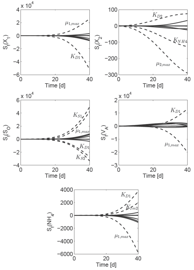
Fig. 1 Numerical solution of the sensitivity function equation (11). Notice that, the parameters subset having the most significant effect on dynamical behavior of AD model (10) are μ1max, μ2max, KD1, KD2, KNH4, KS1, KS2 and KIm2 .
3 Open loop dynamical behavior
In order to compare qualitatively the AD model (10) with literature an example of open loop simulations are shown in Fig. 2. The nominal parameters π0 ϵ π (Table 1) and the nominal operating condition (Table 2) are used for open loop simulation. Two initial condition Φ(t
0) = Φ0 were explored. Case one stands for the following initial condition Φ0 = [0.2, 0.1, 10, 1, 0.5]
T
[g/l]; and case two stands for the initial condition Φ0 = [0.2, 0.1, 10, 2, 0.5]
T
[g/l]. For case one, the trajectories of the states variables converge at desirable state steady
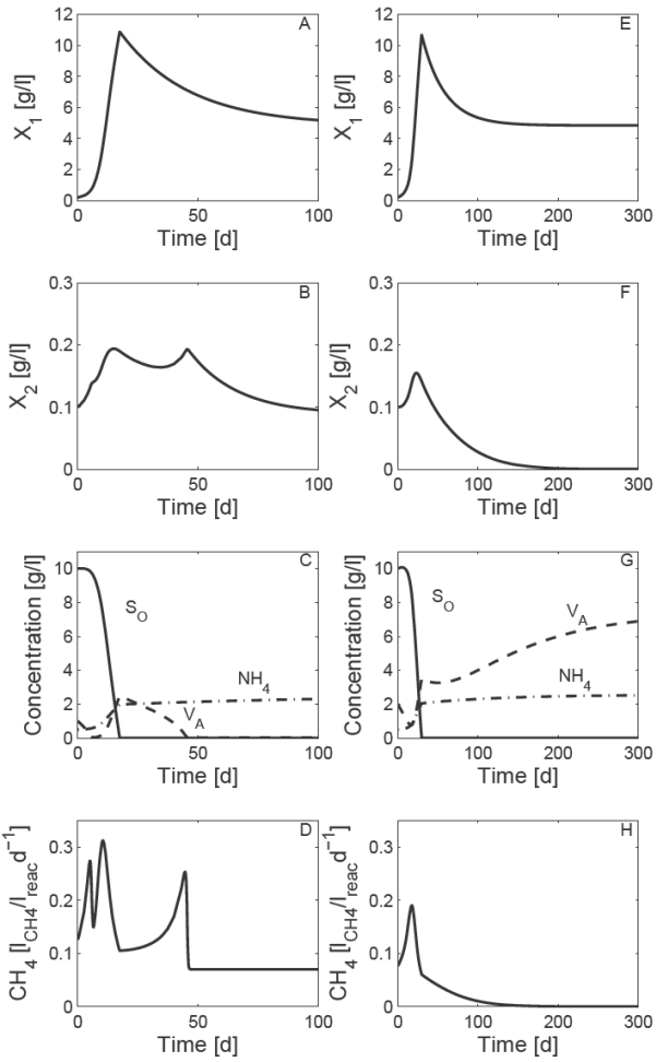
Fig. 2 Numerical solution of the AD model (10) with a set of nominal parameter π0 ϵ Π (Table 1) and nominal operational condition (Table 2). ABCD) case one stand for initial condition Φ0 = [0.2, 0.1, 10, 1, 0.5] T [g/l]. EFGH) case two stand for initial condition Φ0 = [0.2, 0.1, 10, 2, 0.5] T [g/l].
Then, for the same operation condition, it is possible to converge at these two state steady with a set of two different initial conditions. In order to determine convergence to a specific steady state is convenient a dynamical analysis of the equilibrium coordinates. Then, departing from physical properties of the process, equilibrium points stability properties are discussed.
4 The anaerobic digester operating conditions
The following operating conditions can be defined for the anaerobic digester:
• Washout condition. It is said that a digester is operating in washout condition as the biomass isinactive (X 1 = 0, X 2 = 0 for all t ≥ 0) and the remaining states are given by its inlet composition (S O = S O,in, VA = VA,in, NH 4 = NH 4, in for all t ≥ 0). Such condition means that the polluting compounds within the inlet flow are not reduced by the biomass. This operation conditions is undesirable. Then, in order to avoid it, an operational constrain is imposed to inlet flow or dilution rate (D). As a consequence, upper operational value is defined as D* <
• Acidification condition. It is said that a digester is operating in acidification condition (AC) as the only methanogenic biomass is inactive (X 1 > 0, X 2 = 0 for all t ≥ 0), accumulation of VFA is maintained (VA > VA,in ) and some amount of organic matter is treated (S O < S O,in , N H 4 < NH4,in ) for all t ≥ 0.
In other words, this means that the polluting compounds within the wastewater are partially removed by acidogenic bacteria. Accumulation of VFA causes inhibition the methanogenic biomass and only acidogenic biomass is active, as a consequence there is not methane production (QCH4 = 0). It should be note that in real-life experiments, an anaerobic digester can has VFA accumulation with consequent acidification of bioreactor, thus a possible failure (i.e. washout condition). In order to avoid acidification condition, a reduction of dilution rate is done while a methane conversion inefficiency is noticed. This prevents the biomass form short-term stress/inhibition and provides some time to human operators to fix the problem. Note that, in most of real-life experiments it is not identified the upper value restriction of inlet flow or D* which allow to prevent this condition, nevertheless there is a knowledge that this value is lower than Dw .
• Normal operation condition. It is said that a digester is operating in Normal operation condition (NOC) as the biomass is active (X 1 > 0, X 2 > 0 for all t ≥ 0) and the remaining states accomplish S O < S O,in , and VA < VA,in . Then, a fraction of organic matter feeding to AD process is reduced by the acidogenic and methanogenic biomass activity.
5. Dynamic analysis
In order to recognize the possible steady-state solutions for model (10) it is necessary to derive the coordinates of equilibrium. Furthermore, it can be compute equilibrium point and classifier in the sense of stability criterion. Then, such information gives us the main dynamical characteristics of the model. Dynamical analysis of the AD model (10) is performed via linearization principle. Roughly speaking, the procedure consists of the following steps:
to derive the coordinates of the equilibrium Ψ* under a particular considerations from nonlinear AD model (10)
to compute an equilibrium point
to find the Jacobian matrix of the nonlinear model (10)
to compute eigenvalues λ
to corroborate the criteria of locally asymptotically stability. Such that, if all eigenvalues have negative real parts the equilibrium point is locally asymptotically stable. Otherwise, if there is almost one eigenvalue with positive real parts it is an unstable equilibrium point.
First, considering the trivial solution for AD model (10), the coordinate of the equilibrium
 (12)
(12)
Then, for a nominal values and nominal operation condition, the equilibrium point is

Fig. 3 Numerical solution of equilibrium point
From AD model (10) under X
1 = 0 and X
2 ≠ 0 restrictions, four components of the coordinate of equilibrium
 (13)
(13)
and the coordinate of equilibrium for VA is determinate for the solution of the following quadratic equation:
 (14)
(14)
where the coefficient a 1, b 1 and c 1 are:
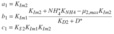 (15)
(15)
As quadratic equation (14) has two solutions

Fig. 4 Numerical solution of eigenvalue
From AD model (10) under X
2 = 0 and X
1 ≠ 0 restrictions, four components of the coordinate of equilibrium
 (16)
(16)
and the coordinate of equilibrium for SO is determined for the solution of the following cubic equation:
 (17)
(17)
where the coefficient a 2, b 2 and c 2 are:
 (18)
(18)
As quadratic equation (17) have two solution
From AD model (10) under X1 ≠ 0 and x2 ≠ 0 restrictions, four components of the coordinate of equilibrium
 (19)
(19)
and the solution of the following cubic equation:
 (20)
(20)
where Eij
(see Appendix A) contain parameters π0 ϵ π and nominal operating condition. As cubic equation (20) have three solution
Table 3 shows the numerical evaluation of the equilibrium points
Table 3 Equilibrium point values
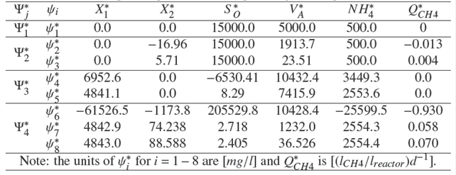
Table 4 depicts the summary of the numerical evaluation of stability analysis. Notice that only the equilibrium points
• Washout condition. It is said that a digester is operating in washout condition as the biomass isinactive(X
1,X
2 =0 for all t ≥ 0)and the remaining states are given by its inlet composition (SO
= SO,in, VA
= VA,in, NH
4 = NH4,in
for all t ≥ 0). This condition arises for
• Acidification condition. It is said that a digester is operating in acidification condition as the only methanogenic biomass is inactive (X
1 > 0, X
2 = 0 for all t ≥ 0), accumulation of VFA is maintained (VA
> VA,in
) and some amount of organic matter is treated (SO
< SO,in, NH
4 < NH4,in
) for all t ≥ 0. This condition arises for 0 < D* <
• Normal operation condition. It is said that a digester is operating in normal operation condition as the biomass is active (X
1, X
2 > 0 for all t ≥ 0) and the remaining states accomplish SO
< SO,in
, and VA
< VA,in
. Then, a fraction of organic matter feeding to AD process is reduced by the acidogenic and methanogenic biomass activity. The Normal operation condition (NOC)
Table 4 Summarize of numerical evaluation of stability analysis. AC means acidification condition and NOC means normal operation condition.
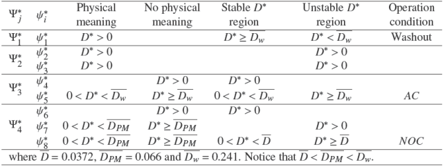
From the results obtained analytically of coordinates of equilibrium
Conjecture 1. Consider the anaerobic digester model
It is clear that the AD model (10) has two locally stable equilibrium point under [Ḏ,
For real-life industrial scale application, the inlet composition is not fixed and it varies in time around a nominal value. Such variation can lead in overload organic matter and possible acidification or failure of AD process (washout). Then, in order to maintain NOC and avoid undesirable operation condition it is necessary a control scheme such that NOC is preserved.
6 Feedback control design
When AD process of OFMSW is used for treatment purposes, the control objective is the regulation of the effluent organic matter despite of fluctuations at the inlet composition (i.e. S O,in , V A,in ). The overall objective in AD process is the conversion of organic matter into a mixture mainly composes of methane and carbon dioxide. Then, in case of non particulate substrate or non-excessively complex organic matter, the limiting step is the conversion of volatile fatty acids into methane (Ariunbaatar et al., 2014; Fernández-Guëlfo et al., 2011). In fact, VFA may accumulate provoking the undesirable acidification operation point and the overall failure of the operation. In this sense, the control problem is formulated to achieve a desirable value of V A through the action of a control scheme.
From AD model (10), it has been shown (Conjecture 1) that
Assumption 1. Only the VA is available for on-line measurement.
Assumption 2. The influent concentrations for SO,in , VA,in and NH4,in are piecewise constants, bounded and uncertain functions.
Assumption 3. The growth kinetics for the acidogenic and methanogenic stages are: smooth, bounded and uncertain functions.
Assumption 4. The dilution rate is constrained by saturation function:
 (21)
(21)
where the bounds Ḏ and
Assumption 1 is not restrictive in sense that there is available technology to measure on-line VA by direct relationship with volatile fatty acid (VFA) or indirectly, throughout linear function with another key variable as total alkalinity. Notice that under Assumption 1-3 the controller must be restricted. For practical D is common restricted to avoid washout condition; nevertheless for AD model (10)
In order to show the control problem is solvable a PI controller is designed. First, a linear nominal plant is derive (Khalil, 2002) from nonlinear AD model (10) at equilibrium point
 (22)
(22)
where u is the input variable D and the output variable y is V A . Then, with the dynamical characteristics of the nominal plant a controller is obtained:
 (23)
(23)
where K p,0 is the proportional constant and K i,0 is the integral constant. Here, since nominal process model (22) is available, a classical tuning method is used in order to obtain the values of K0 = [K p,0 ,K i,0 ]. Using Ziegler-Nichols (Yu, 2002) tuning rule a set of constants are obtained K0 = [K p,0 ,K i,0 ] = [0.0087, 0.31102].
The Fig. 6 shows the numerical results of the performance of the PI controller K0 under set point changes and load disturbances (see Fig. 5) on the nonlinear AD model (10). The load disturbances are simulated with changes in S O,in among the nominal inlet concentration S O,in = 15 [g/l] (Table 2). The PI controller performance remains acceptable throughout the simulations; nevertheless it is deteriorated at the set point changes. As set point changes the control input (dilution rate) can lead to undesirable operation condition of the AD process such a saturation, which it can not be accepted in practice. In order to show the performance of the controller under changes of tuning rules, a change in proportional parameter is explored under two additional controllers K1 = [0.75K p,0 , K i,0 ] and K2 = [2K p,0 , K i,0 ].
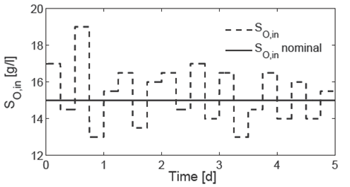
Fig. 5 Inlet concentration disturbances S O,in for closed-loop simulation of the controlled system. The inlet concentration S O,in is fixed among the nominal inlet concentration S O,in = 15 [g/l] (Table 2).

Fig. 6 Closed-loop behavior of the controlled system under inlet disturbances (see Fig. 5). A) output V
A
concentration is maintained close of changes in set point concentration among the coordinate of equilibrium point
The Fig. 6 shows the numerical results of the performance of the PI controller K1 and K2 under inlet disturbances (see Fig. 5). Controller K0 shows less convergence and major control effort with respect to controller K1 and K2. The controller K2 shows less control effort and faster convergence to V A,ref with respect to controller K0 and K1. Despite of improvement with a trial an error tuning schema, robust control strategies should be explorer.
7 Concluding remarks
A simple model of AD process of OFMSW is proposed for control process. The model includes adequate description of: (i) two metabolic stages such as acidogenesis and methanogenesis are considered; (ii) inhibition product is included; (iii) ionic equilibrium is assumed.
The AD model (10) predicts washout, acidification, and normal operation condition. These operation conditions were addressed for existence and stability criterion. Note that AD model predict acidification condition, it is important issue such that it can be used to obtain confidence intervals of operation, process design and experimental strategies with less disruption.
Under dynamical analysis, it was possible to asses a general framework to synthesize a classical PI controller. Numerical simulations showed that under nominal parameter is possible achieve stabilization of no linear AD process of OFMSW under inlet disturbances. For some change of set point and persistent disturbances the controller present performance organic matter degradation, for these cases is necessary a different framework in order to face this issue; indeed, results in this direction will be reported elsewhere.


