Simulación y control

 

Model for the development of a low cost thermal mass flow meter

 

Modelo matemático para el desarrollo de un medidor térmico de flujo másico de bajo costo

 

C. García-Arellano^1* and O. García-Valladares²

 

¹ Posgrado en Ingeniería, Energía, Universidad Nacional Autónoma de México (UNAM), Privada Xochicalco S/N, Temixco, 62580 Morelos, México.*Corresponding author. E-mail: rasecgarella@hotmail.com Tel. (52)(777)3250046 ext. 29746

² Centro de Investigación en Energía (CIE), Universidad Nacional Autónoma de México (UNAM), Privada Xochicalco S/N, Temixco, 6225580 Morelos, México.

 

Received 05 of February 2009
Accepted 25 of September 2011

 

Abstract

This paper presents the mathematical model for the development of a water mass flow meter. Its operation principle is based on a relation between a constant input power (heat flow) provided to the system and the increase of temperature in the test section. A numerical model of the thermal and fluid dynamic behavior of the thermal mass flow meter is carried out ; the governing equations (continuity, momentum and energy) inside the tube together with the energy equation in the tube wall and insulation are solved iteratively in a segregated manner. The parametric study developed with the numerical model includes the tube diameter, tube length, and the power supply to the system, with the numerical results obtained and taking into account some restrictions on the system, the final design of the system has been obtained and constructed. A test procedure was carried out to show the technical feasibility of this system and an error of mass flow rate of ± 0.55 % was obtained. In relation to the cost, the errors of experimental measurement are acceptable if they are compared with some of the more common available commercial systems with much higher cost.

Keywords: design, thermal mass flow meter, heat transfer, numerical model.

 

Resumen

Se presenta el modelo matemático para el desarrollo de un medidor de flujo másico. Su principio de operación esta basado en una relación entre el flujo de calor suministrado a la sección de prueba y la diferencia de temperaturas entre la entrada y la salida. Un modelo numérico del comportamiento térmico y fluido-dinámico del medidor térmico de flujo másico es desarrollado; las ecuaciones gobernantes dentro del tubo (continuidad, momentum y energía) junto con la ecuación de la energía en la pared del tubo y el aislante han sido resueltas iterativamente y de una forma segregada. El estudio paramétrico desarrollado con el modelo numérico incluye el diámetro, longitud del tubo así como la potencia suministrada al sistema; con los resultados numéricos obtenidos y tomando en cuenta algunas restricciones sobre el sistema, el diseño final se obtuvo y se construyó. Se llevó a cabo un procedimiento de pruebas para mostrar la factibilidad técnica de sistema y se encontró un error en la medición de flujo de ±0.55%. En relación con el costo de construcción, los errores de las mediciones experimentales son aceptables si se comparan con algunos de los medidores comerciales más comúnmente usados de mayor precio.

Palabras clave: diseño, medidor térmico de flujo másico, transferencia de calor, modelo numérico.

 

1 Introduction

The measurement and control of mass flow rate is critical in many industrial and experimental applications. Flux is defined as: the amount of mass flow through an area per unit time. Currently there are a wide variety of commercial flow meters, which can be constructed and designed for different operating conditions. Its classification is based on their operation principle, as shown in (Table 1). Particularly, the cost is an important factor to be considered in instrument selection.

There are two methods to measure flow: direct and indirect. The second method was applied frequently by a simultaneous combination of volumetric flow and density meters, both depend on pressure and temperature. Nevertheless, this is not accurate since errors exist in the measurement instruments. Therefore, direct measurement methods are preferable in industrial processes (Zhang et al., 2006). Thermal mass flow meters are widely used in industry in order to measure small flows.

Two techniques are commonly employed: the first is to provide a constant input power to a section of tubing and measure the temperature of the tube on both sides of the heated section, the flow skews the temperature distribution of the tube such that the downstream temperature is larger than the upstream value. This measured difference is linearly dependent upon mass flow rate. The second technique, heats the tube by maintaining a constant temperature independent of flow, in this way the amount of power required to maintain the constant tube temperature is then proportional to the mass flow rate in the tube. For this work the first technique is used.

To understand the operation principle of thermal mass flow meters, the term heat capacity must be considered; this is defined as the quantity of heat required to raise the temperature a specific numbers of degrees. In previous years several evaluations of this type of systems have been developed. For example, experimental results for thermal mass flow meters working under different conditions and using different types of heaters arrangements have been reported by (Hawk and Baker, 1968; Komiya et al., 1988; Hinkle and Mariano, 1991; Tison, 1996; Toda et al., 1998; Rudent et al., 1998; Kim and Jang, 2001; Viswanathan et al., 2002; Viswanathan et al., 2002; Kim et al., 2007; Han et al., 2005); some authors have developed numerical models of the system in order to represent the phenomenology of it, for example: (Kim and Jang, 2001; Kim et al., 2007; and Han et al., 2005).

The objective of this work is to present the development of a water mass Flow Meter (FM) of low cost. For this purpose, a numerical simulation model of the thermal and fluid dynamic behavior of the thermal mass flow meter has been carried out.

In this paper, the operating principle will be explained first; then the numerical model and numerical algorithm are explained and a numerical parametric study has been carried out in order to design the system; finally, the experimental set up and comparisons of numerical solution and polynomial function (developed in order to obtain the mass flow rate) with experimental data are shown.

 

2 Operating principle

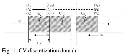
A mass flow rate enters to the test section in the experimental set up, with inlet temperature (T_i), pressure (p_i) and velocity (v_i); as it moves forward, its initial conditions change due to the heat transfer with a constant electrical resistance and the shear stress with the tube wall until reaching its outlet conditions: temperature (T_n), pressure (p_n) and velocity (v_n). This is shown in Fig. 1.

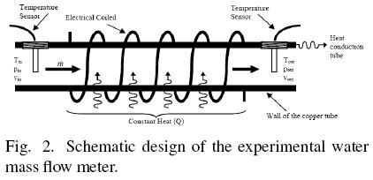
Its operation principle is based on the First Law of Thermodynamics. During the process, water mass flow to the test section; this section is heated with a constant electric coil around the tube external surface. The water temperature is measured by two temperature sensors at the inlet and outlet sections. Thus, the mass flow rate is inversely proportional to the temperature difference registered by the sensors. The schematic is shown in Fig. 2.

 

3 Mathematical model

A computational algorithm has been carried out in order to obtain the thermal and fluid dynamic behavior of the thermal mass flow meter and in order to design and optimize it. The mathematical model was divided in three subroutines: fluid flow inside tube, heat transfer in a tube with constant input heat power supply in its external surface and heat transfer in a tube with insulation.

3.1 Spatial and temporal discretization

Fig. 3, shows the spatial discretization of a double pipe heat exchanger. The discretization nodes are located at the inlet and outlet sections of the CVs in the fluid flow, while the discretization nodes are centred in the CVs in the tube wall and insulation. The fluid has been divided into n_z volumes (i.e., n_z+1 nodes). The tube wall has been discretized into n_z control volumes of length Δ_z. The insulation are discretized into n_z x n_r control volumes of length Δ_z and width Δr, where Δr = (D₂ - DO/₂ for j = 1 and Ar = (D₂- D₂)/(2(n -1))for j > 1.

The transitory solution is performed every time step Δt. Depending on the time evolution of the boundary conditions, a constant or variable value of Δt can be selected.

3.2 Mathematical model of fluid flow inside tube

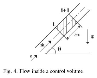
In this section the mathematical formulation of the fluid flow inside a characteristic CV of a tube is presented (see Fig. 4), where 'i' and 'i+1' represent the inlet and outlet sections respectively.

Taking into account the characteristic geometry of tube (diameter, length, roughness, angle, etc.), the governing equations have been integrated assuming the following assumptions:

• One-dimensional flow: p(z, t), h(z, t), T(z, t),...

• Fluid: pure and mixed substances.

• Non-participant radiation medium and negligible radiant heat exchange between surfaces.

• Axial heat conduction inside the fluid is neglected.

• Constant internal diameter and roughness.

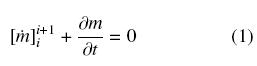
The semi-integrated governing equations over the above mentioned finite CV, have the following form (García-Valladares et al., 2002):

• Continuity:

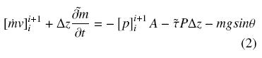
• Momentum:

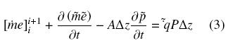
• Energy:

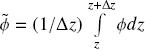
where represents the integral volume average of a generic variable φ over the CV and its arithmetic average between the inlet and outlet of the CV. The subscript and superscript in the brackets indicate 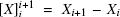, i.e., the difference between the quantity X at the outlet section and the inlet section.

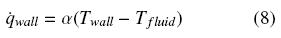
In the governing equations, the evaluation of the shear stress is performed by means of a friction factor /. This factor is defined from the expression: τ = Φ(f/4)(G²/2ρ), where Φ is the two-phase factor multiplier. The heat transfer through the tube wall and fluid temperature are related by the convective heat transfer coefficient α, which is defined as: α = q_wall/(T_wall- T_fluid).

3.2.1 Evaluation of empirical coefficients

The mathematical model requires local information about friction factor f and the convective heat transfer coefficient α. This information is generally obtained from empirical or semi-empirical correlations. After comparing different empirical correlations presented in the technical literature, we have selected the following to obtain the results here presented: the convective heat transfer coefficient is calculated using the Nusselt and the Gnieliski equations (Gnielinski, 1976), for laminar and turbulent regimes respectively; and the friction factor is evaluated from the expressions proposed by Churchill (1977).

3.2.2 Discretization equations of flow inside tubes

The discretized equations have been coupled using a fully implicit step by step method in the flow direction. From the known values at the inlet section and guessed values of the wall boundary conditions, the variable values at the outlet of each CV are iteratively obtained from the discretized governing equations. This solution (outlet values) is the inlet values for the next CV. The procedure is carried out until the end of the tube is reached.

For each CV, a set of equations is obtained by a discretization of the governing equations (1)-(3). In the section mathematical formulation, the governing equations have been directly presented on the basis of the spatial integration over finite CVs. Thus, only their temporal integration is required. The transient terms of the governing equations are discretized using the following approximation: ∂φ/∂T ≅ (φ - φº)/Δt, where φ represents a generic dependent variable (φ = h, p, T,p,...); superscript "o" indicates the value of the previous instant.

The averages of the different variables have been estimated by the arithmetic mean between their values at the inlet and outlet sections, that is:_i ≅ _i ≡ (φ_i +φ_i+1)/2.

Based on the numerical approaches indicated above, the governing equations (1)-(3) can be discretized to obtain the value of the dependent variables (mass flow rate, pressure and enthalpy) at the outlet section of each CV. The final form of the governing equations is given below.

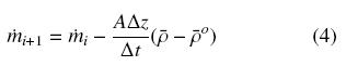
The mass flow rate is obtained from the discretized continuity equation,

The discretized momentum equation is solved for the outlet pressure,

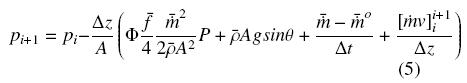
From the energy equation (3) and the continuity equation (1), the following equation is obtained for the outlet enthalpy:

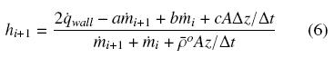
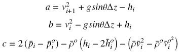
where

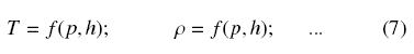
Temperature and thermophysical properties are evaluated using matrix functions of the pressure and enthalpy, refilled with the refrigerants properties evaluated using the REFPROP v.8.0 program (REFPROP, 2007):

The above mentioned conservation equations of mass, momentum and energy together with the thermophysical properties, are applicable to transient flow. Situations of steady flow are particular cases of this formulation. Moreover, the mathematical formulation in terms of enthalpy gives generality of the analysis (only one equation is needed for all the regions) and allows dealing with cases of mixtures of fluids.

3.2.3 Boundary conditions

• Inlet conditions: the boundary conditions for solving a step by step method directly are the inlet mass flux m_in, pressure p_in and temperature Tin. From temperature and the pressure, enthalpy (our dependent variable) is obtained. Other boundary conditions such as (p_in, p_out) or (T_in, T_out) can be solved using a Newton-Raphson algorithm. The method is based on an iterative process where the inlet mass flow rate is updated until global convergence is reached.

• Solid boundaries: The wall temperature profile in the tube must be given. These boundary conditions are expressed in the energy equation in this form:

3.2.4 Solver

In each CV, the values of the flow variables at the outlet section of each CV are obtained by solving iteratively the resulting set of algebraic equations (continuity, momentum, energy and state equations mentioned above) from the known values at the inlet section and the boundary conditions. The solution procedure is carried out in this manner, moving forward step by step in the flow direction. At each cross section, the shear stresses and the convective heat fluxes are evaluated using the empirical correlations obtained from the available literature (see Evaluation of Empirical Coefficients). The transitory solution is iteratively performed at each time step. If a transient case is analyzed, depending on the time evolution of the boundary conditions, a constant or variable value of Δt can be selected.

Convergence is verified at each CV using the following condition:

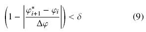
where φ refers to the dependent variables of mass flow rate, pressure and enthalpy; and φ* represents their values at the previous iteration. The reference value Δφ is locally evaluated as φ_i+₁ - φ_i. When this value tends to be zero, Ap is substituted by φ_i.

3.3 Mathematical model of a tube with constant input heat power supply in its external surface

The conduction equation has been written assuming the following hypotheses: one-dimensional transient temperature distribution and negligible heat exchanged by radiation. A characteristic CV is shown in Fig. 5, where 'P' represents the central node, 'E' and 'W' indicate its neighbours. The CV-faces are indicated by 'e, 'w', 'n' and 's'.

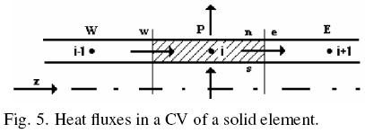
Integrating the energy equation over this CV, the following equation is obtained:

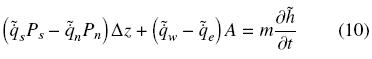
where is evaluated using the respective convective heat transfer coefficient and temperature of the fluid flow, is the constant heat power supply by electrical resistance, and the conductive heat fluxes are evaluated from the Fourier law, that is: 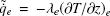and .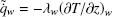

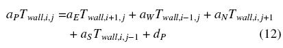
The following equation has been obtained for each node of the grid:

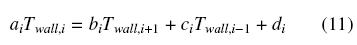
where the coefficients are,

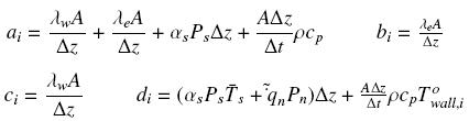
The coefficients mentioned above are applicable for 2 ≤ i ≤ n_z — 1; for i=1 and i = n_z adequate coefficients are used to take into account the axial heat conduction or temperature boundary conditions. The set of heat conduction discretized equations is solved using the algorithm TDMA (Patankar, 1980).

3.4 Mathematical model of a tube with insulation

The tube wall is solved in a similar way as described in the previous section for the internal tube. The conduction equation for the insulation has been written assuming transient axisymmetric temperature distribution and negligible heat exchanged by radiation with the external ambient. The north and south interfaces are evaluated from the Fourier law, except in the tube-insulation interface (where a harmonic mean thermal conductivity is used) and in the insulation-ambient interface (where the heat transfer by natural convection is introduced).

The following equation has been obtained for each node of the grid:

where the coefficients are,

The coefficients mentioned above are applicable for 2 ≤ i ≤ n_z - 1 and 2 ≤ j ≤ n_r - 1; for the nodes in the extremes (see Fig. 3) the following considerations have been applied:

• For j = 1 forced convection is considered in the south face, tube thermal conductivity in east and west faces and insulation thermal conductivity in north face, all these evaluated to the mean temperature between the nodes that separated them.

• For j = n_r natural convection with the ambient is considered [using the correlation developed by Raithby and Hollands (Raithby and Hollands, 1975) and also the conduction through the insulation external part of thick equal to Δr/2, with thermal conductivity evaluated to the node temperature.

• For i = 1 and i = n_z adequate coefficients are used to take into account the axial heat conduction or temperature boundary conditions.

 

4 Numerical algorithm

The solution process is carried out on the basis of a global algorithm that solves in a segregated manner the fluid low inside tube, heat transfer in a tube with constant input heat power supply in its external surface and heat transfer in a tube with insulation. The coupling between the three main subroutines has been performed iteratively following the procedure:

• For fluid flow inside tube, the equations are solved considering the tube wall temperature distribution as boundary condition, and evaluating the convective heat transfer and fluid temperature in each CV.

• For heat transfer in a tube with constant heat power supply in its external surface, the temperature distribution in the tube is recalculated using the fluid low temperature and the convective heat transfer coefficients evaluated in the preceding steps and considering the constant input heat power supply by the electric resistance and the ambient thermal losses calculated in the next step.

• For heat transfer in a tube with insulation, the ambient thermal losses are calculated considering the tube wall temperature distribution calculated in the preceding step and the insulation thickness and the natural convective heat transfer coefficients evaluated in the external ambient.

The global convergence is reached when between two consecutive loops of the three main subroutines a strict convergence criterion is verified for all the CVs in the domain.

The mass low rate through the systems is solved using a Newton-Raphson algorithm with the following boundary condition (T_in, T_out) registered by the thermocouples in the experimental set up. The method is based on an iterative process where the inlet mass low rate is updated until global convergence is reached.

Based on the above mentioned mathematical model and numerical algorithm, a code has been developed for the detail numerical simulation of the thermal and fluid dynamic behavior of the thermal mass low meter. The numerical results obtained by the mathematical model for this particular mass flow meter are presented in the design and optimization and the experimental validation sections. All numerical results obtained are grid independence solutions.

The numerical model developed is based on the applications of governing equations and used general empirical correlations (any correction factor has been used); for this reason, it is possible to make use of it to other fluids, mixtures and operating conditions; it allows using the model developed as an important tool to design these kinds of systems.

 

5 Design of the thermal mass flow meter

Based on the mathematical model of the thermal and fluid dynamic behavior of the thermal mass low meter carried out, the design of this system is described in this section.

The main objective is to obtain a water mass flow meter of low cost with a good performance for the user (i.e. reasonable mass low rate error, low pressure drop, reasonable consume of energy, etc.). In order to reach this objective, the numerical model has been used in order to obtain a parametric study of this system.

The following restrictions have been considered in order to design and optimize the system: a) the range of the mass flow rate was fixed from 3 to 17 kg/min; b) the Reynolds number over the entire range of mass flow rate must be in the turbulent region (higher than 5000 in order to be sure that the system is not working in the laminar or transition region were the heat transfer coefficients decrease significant and it can affect the system performance); c) due to the temperature sensors used in the system have an accuracy of ±0.2 ºC, the minimum difference of temperature between the inlet and outlet section is 0.2 ºC; d) material of the tube with high thermal conductivity; e) low pressure drop in the system is required in order to not perturb significantly the process where the system can be install.

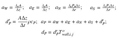
The parametric study developed includes the tube diameter, tube length, and the power supply to the system shown in (Table 2). For all the cases, the numerical model has fixed the following parameters: inlet water temperature (25 ºC), ambient temperature (30 ºC), thickness of flexible foam insulation (", 19.05 mm) for all the tube diameters and copper tube (due to its high thermal conductivity).

The average Reynolds numbers obtained by the numerical model for the different tube diameter considering the lowest mass flow rate (3 kg/min) are: 8939 (for "), 5167 (for ") and 3587 (for "); the pressure drop obtained for highest mass flow rate (17 kg/min) and the highest length (0.75 m) was: 31.6 kPa, 2.3 kPa and 0.4 kPa respectively or 8.95 W, 0.65 W and 0.11 W of power consumption (assuming that the power consumption is approximately equal to pressure drop multiplied by the mass flow rate and divided by the fluid density). According to these results and the restrictions mentioned above, the " nominal diameter tube has been discarded due to the high pressure drop obtained and the " nominal diameter has been discarded due to the small Reynolds number obtained that can produce that the system can operate in the transition zone between laminar and turbulent flow.

Fig. 6 shows the increment of the water temperature in function of the tube length and heat power supply for the " tube nominal diameter. According to the restriction of minimum temperature difference between the inlet and outlet section of 0.2ºC the heat powers of 210 and 270 W has been eliminated and due to save energy in the system operation the 330 W heat power supply has been selected.

Due to the electrical resistance found commercially has a resistance of 1.75 Ω/m with a diameter of 5 mm, the length necessary to reach 330 W of heat power is 3.08 m (considering the electrical energy supply in Mexico of 127 V a.c. and in order to not used voltage regulators); this length is impossible to be coiled in the 0.25 m length tube and the 0.75 m length tube has been discarded in order to obtain a system that can be mounted in an easy way (reducing space) in experimental systems.

The final design obtained for the thermal mass flow meter by the numerical analysis has the following characteristics: " nominal diameter of copper tube, 0.5 m length, 330 W of heat power and a thickness of the flexible foam insulation of ".

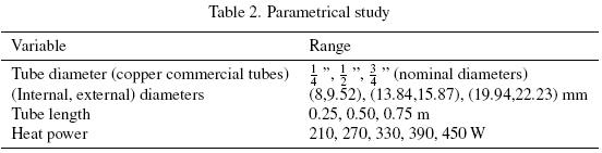
With the numerical model and the final geometry conditions given above, the following polynomial equation has been developed in order to calculate theoretically the mass flow rate of the system in function of the temperature difference between the inlet and outlet section and the power supply by the electrical coiled:

 

6 Experimental setup

Based on the numerical model the final design of the thermal mass flow meter mentioned above was obtained and constructed. A domestic Mexican voltage is used to obtain this power supply without using voltage regulators.

Fig. 7 shows a general diagram of the experimental set up. The electrical power supplier is a flexible electrical resistance of 3.08 m with a diameter of 5 mm coiled over the external tube wall in order to maintain a constant heat flux; two sensors of temperature (thermistors with an accuracy of ±0.2°C) were installed at the inlet and outlet sections.

A Coriolis equipment with an accuracy of ±0.1% (Coriolis, Endress Hausser Instruction Manual, 2000) of mass flow rate was installed on the work line in order to determine the water mass flow rate across the test section; this error is taken into account in the experimental measurements; but the error is too small to affect significantly the experimental results.

At the end of the test section a sight flow indicator was instafled in order to visualize the flow behavior. Table 3 presents the characteristics of the experimental thermai mass flow meter developed.

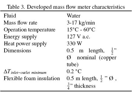
All experimental data are registered with an acquisition data logger. Computer software was developed and tested in order to register, analyze and process all the involved variables.

The minimum distance to have a fully developed flow and obtain reliable results is 12 diameters to the entrance and ¹⁰ diameters at outiet section (for the system devektped 0.152 m and 0.127 m respectively). This distance was taken into account in the experimental set up. Major obstructions such throttied vaives, eibows or pumps wifl require longer straight runs.

 

7 Test procedure

The objective of this test procedure is to determine experimentally the mass flow rate across the section test and its percentage of error with respect to a Coriolis mass flow meter. The characteristics to take into account include (Belforte et al., 1997): type of fluid (liquid or gas), physical properties to be measured, working conditions, accuracy and precision.

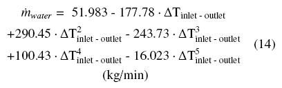
Three characteristics polynomials were experimentally obtained for each one of the water inlet temperatures tested by means of the temperature difference registered by the inlet and outlet temperature sensors and the mass flow meter measured by the Coriolis instrument.

For inlet water temperature of 20º C

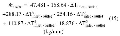
For inlet water temperature of 40º C

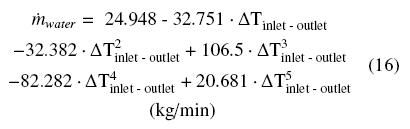
For inlet water temperature of 60º C

These five order polynomial equations have been integrated into the developed software to be validated with new experimental data in order to estimate the repeatability and error of this system. For intermediate water inlet temperatures a linear interpolation of these polynomial equations is used.

7.1 Experimental validation

The experimental test begins with the watercirculation from storage tank 1 to 2 (see Fig. 7). Previously, inlet water temperature has been fixed by an electrical heat supplier installed inside the storage tank 1. The water flow enters into the section test, where a constant heat flux is applied through all the external surface of the tube wall, two sensors register the temperature difference (ΔT_inlet-outlet) that is used in the polynomial equation according to each case.

Experimental values were registered each 5 s; twenty tests were performed for each temperature in order to verify the accuracy and error of this system. Mass flow rate test validation begins with 3 kg/min and it is increased in 1 kg/min until reach 17 kg/min. The steady state condition for each one of the experimental points is reached once the (ΔT_inlet-outlet) is maintained constant in ±0.2°C; for low flows (3-8 kg/min) the stabilization time required is approximately 30 s, meanwhile for high flows (9-17 kg/min) the stabilization time is reduced to approximately 15 s.

With flows higher than 18 kg/min, the measurement errors (ΔT_{inlet-outlet, minimum}) are higher than the difference temperature between inlet and outiet temperature sensors, for this reason, the mass low range was limited until 17 kg/min in experimental tests. In order to evaluate mass flow rate over 18 kg/min a higher heat power had to be applied or a by-pass (that will be explained below) can be impiemented.

For the comparison with experimental data, the foiiowing definitions are used:

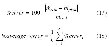
where k is the number of data points and m_real is the measurement obtained by the Coriolis mass flow meter.

Fig. 8 presents the experimental results for a test with an inlet water temperature of 19.5 ^°C; in this case an average error of ± 0.46% and a maximum error of ±0.98% of mass flow rate are observed with a standard deviation of 0.04. In the experimental tests, the error bars represent the standard deviation for each one of the measured points.

Fig. 9 presents the mass flow rate obtained by a linear interpolation for two polynomial equations (20 ^°C and 40 ^°C respectively) for the inlet water temperature of 24.4 ^°C. With this interpolation, mass flow rates with a smaller degree of uncertainty can be obtained. From this figure it can be seen that the experimental flows registered by the linear interpolation adjust fairly good to the mass flow rate register by the Coriolis instrument. An average error of ± 0.46% is observed with a maximum error of ±0.84% of mass flow rate and a standard deviation of 0.034.

Fig. 10 shows the experimental mass flow rate test with inlet water temperature of 40.4 ^°C, an average error of ±0.31%, with a maximum error of ±0.83% and a standard deviation of 0.047 have been obtained.

For the case presented in Fig. 11, an inlet water temperature of 60.1 ^°C was used, an average error of ±0.91%, a maximum error of ±1.91% of mass flow rate and a standard deviation of 0.06 are observed. Although the experimental results obtained in this case from the corresponding polynomial equation have a good agreement with the measured real mass flow rate, errors higher than the previous tests (figs. 8-10) (9) can be observed; these errors can be diminished with a more compact fit of the flow curve calibration. In spite of the registered errors, the average error can be considered acceptable.

The repeatability of the mass flow meter readings was checking and fairly good results have been obtained during the test procedure.

In Fig. 12 the calculated mass flow rate profiles (represented by the numerical model considering 330 W of constant heat flux and the prediction limits) are compared with the experimental mass flow rate obtained by the Coriolis system. It is found that an error of +0.1°C in the two sensors that register the temperature difference (AT_inlet-outlet) has an important effect in the band of results obtained by the numerical model. On the other hand, the AT_inlet-outlet error band improved the matching between the simulated and measured mass flow rate. In conclusion, the existing deviations between the numerical model and the experimental results are due principally to the error in the two sensors that register the temperature difference (AT_inlet-outlet) and in a minor degree to thermal losses to the environment, losses by conduction in tubes and connections and uncertainties of measurement instruments. Even so, numerical results present good tendencies with the experimental ones.

The avarage error between the numerical model and the experimental results is ± 7.41% of mass flow rate. The error is reduced due to the temperature sensors accuracy ± 0.2°C. The error is diminished when AT_inlet-outlet increases; i.e. for the case of an interval higher than 0.6°C the error diminished to ±5.38%, and for an interval higher than 1.0°C the error is ±4.46%.

When the experimental results obtained by means of the polynomial equations are compared to the real value measured by the Coriolis mass flow meter, an average error of ±0.55% is obtained; this error is acceptable considering the construction cost.

Experimentally, the measured mass flow rates can be increased (to values higher than 17 kg/min) with the same principle without increasing the input power, by means of a by-pass in the test section; thus, there is a proportional correspondence of the total mass flow rate measured in the experimental section, respect to the mass flow rate that crosses the by-pass section (k), as shown in Fig. 13.

 

8 Accuracy and cost of the experimental mass flow meter compared to commercial flow meters

The simple design of the experimental thermal mass flow meter developed produces a cheap system without movable parts. The device can be a viable and competitive option in the market according to the working conditions and mass flow rate to be used. In relation to the cost, the errors of experimental measurement are acceptable if they are compared with some of the more common commercial systems; for example, a comparison of the developed mass flow meter with an electromagnetic or positive displacement mass flow meter available in the market that have similar uncertainties in mass flow rates measurement (±0.55%), shows that the system developed reduced the price between 10 and 11 times. Thus, it is demonstrated that an elevated investment is not necessary in order to obtain reliable results. Moreover, the characteristic polynomial equation obtained can be implemented in an easy way in a chip.

 

Concluding remarks

An experimental thermal mass flow meter of low cost has been developed; its operation is based on the solution of governing equation presented in the numerical model section.

With the parametric study developed with the numerical model and taking into account some restrictions on the system, the final design of the system has been obtained and constructed.

The experimental mass flow meter has been developed in a mass flow rate range from 3 to 17 kg/min. Three polynomial equations at 20 ºC, 40 ºC and 60 °C have been developed in order to characterize the experimental mass flow meter, these equations are based on the inlet-outlet temperatures registered and the heat power supplied. The application of the polynomial equations allowed obtaining directly the mass flow rate across the test section. There was no need of measuring other physical properties; therefore no additional equipment was required. In addition, the developed flow meter has no movable parts so it will not have mechanical failures and the polynomial equation can be implemented in an easy way in a chip.

The experimental average error obtained with the developed system is ±0.55% of mass flow rate, this error is acceptable when construction cost and measure quality are compared.

The numerical model developed is based on the applications of governing equations and used general empirical correlations (any correction factor has been used); for this reason, it is possible to make use of it to other fluids, mixtures and operating conditions (including gas or two-phase flow); it allows using the model developed as an important tool to design these kinds of systems.

 

Acknowledgements

This work had been financed by CONACyT project U44764-Y. The authors thank Dr. V.H. Gomez for the technical support, Dr. Jorge Andaverde for the contribution in the study of the experimental errors and to CONACyT, Mexico, for the support provided for the student scholarship 173571.

 

Nomenclature

A cross section area, m²

c_P specific heat at constant pressure, J kg^-1 K^-1

D tube diameter, m

e specific energy (h+v²/2+gzsin θ), J kg^-1

f friction factor

^g acceleration due to gravity, m s^-2

G mass velocity, kg m^-2 s^-1

h enthalpy, J kg^-1

k number of data points

L length, m

m mass, kg

m mass flow rate, kg s^-1

n number of control volumes

^p pressure, Pa

P perimeter, m

^q heat flux per unit area, W m^-2

Q heat flux, W

t time, s

T temperature, K

v velocity, m s^-1

z axial direction, m

Greekletters

α heat transfer coefficient, W m^-2 K^-1

Δr radial discretization step, m

Δt temporal discretization step, s

ΔT temperature difference, K

Δz axial discretization step, m

Ø tube diameter, m

Φ two-phase frictional multiplier

θ angle, rad

λ thermal conductivity, W m^-1 K^-1

ρ density, kg m^-3

τ shear stress, Pa

Subscripts

e east

i inlet

n north

pred predicted

s south

w west

Superscripts

~ integral average over a CV:

° previous instant

* previous iteration

 

References

Belforte G., Carello M., Mazza L. and Pastorelli S. (1997). Test bench for flow rate measurement: calibration of variable area meters. Measurement 20, 67-74.         [ Links ]

Churchill S.W. (1977). Friction equation spans all fluid flow regimes. Chemical Engineering 84, 91-92.         [ Links ]

Coriolis, Endress Hausser Instruction Manual (2000).         [ Links ]

García-Valladares O., Pérez-Segarra C.D. and Oliva A. (2002). Numerical simulation of capillary-tube expansion devices behaviour with pure and mixed refrigerants considering metastable region. Part I: Mathematical formulation and numerical model. Applied Thermal Engineering 22, 173-182.         [ Links ]

García-Valladares O., Pérez-Segarra C.D. and Rigola J. (2004). Numerical simulation of double-pipe condensers and evaporators. International Journal of Refrigeration 27, 656-670.         [ Links ]

Gnielinski V. (1976). New equations for heat and mass transfer in turbulent pipe and channel flow. International Chemical Engineering 16, 359-368.         [ Links ]

Han Y., Kim D. K. and Kim S. J. (2005). Study on the transient characteristics of the sensor tube of a thermal mass flow meter. International Journal of Heat and Mass Transfer 48, 2583-2592.         [ Links ]

Hawk C. E. and Baker W. C. (1968). Measuring small gas flows into vacuum systems. The Journal of Vacuum Science and Technology 6, 255-257.         [ Links ]

Hinkle L. D. and Mariano C. F. (1991). Toward understanding the fundamental mechanisms and properties of the thermal mass flow controller. The Journal of Vacuum Science and Technology A 9, 2043-2047.         [ Links ]

Kim D. K., Han I. Y. and Kim S. J. (2007). Study on the steady-state characteristics of the sensor tube of a thermal mass flow meter. International Journal of Heat and Mass Transfer 50, 1206-1211.         [ Links ]

Kim S. J. and Jang S. P. (2001). Experimental and numerical analysis of heat transfer phenomena in a sensor tube of a mass flow controller. International Journal of Heat and Mass Transfer 44, 1711-1724.         [ Links ]

Komiya K., Higuchi F. and Ohtani K. (1988). Characteristics of a Thermal Gas Flowmeter. Review of Scientific Instruments 59, 477-479.         [ Links ]

Patankar S.V. (1980). Numerical Heat Transfer and Fluid Flow. New York: McGraw-Hill.         [ Links ]

Raithby G. D. and Holland G. T. (1975). Advances in Heat Transfer, ed. by Irvine and Hartnett, vol. 11, Academic Press, New York.         [ Links ]

REFPROP v8.0, Reference fluid thermodynamic and transport properties. NIST Standard Reference Data Program, USA, 2007.         [ Links ]

Rudent P., Navratil P., Giani A. and Boyer A. (1998). Design of new sensor for mass flow controller using thin film technology based on an analytical thermal model. The Journal of Vacuum Science and Technology A 16, 3559-3563.         [ Links ]

Tison S. A. (1996). A critical evaluation of thermal mass flow meters. The Journal of Vacuum Science and Technology A 14, 2582-2591.         [ Links ]

Toda K., Maeda Y., Sanemasa I., Ishikawa K. and Kimura N. (1998). Characteristics of a thermal mass-flow sensor in vacuum systems. Sensors and Actuators A 69, 62-67.         [ Links ]

Viswanathan M., Rajesh R. and Kandaswamy A. (2002). Design and development of thermal mass flowmeters for high pressure applications. Flow Measurement and Instrumentation 13, 95-102.         [ Links ]

Viswanathan M., Kandaswamy A., Sreekala S. K. and Sajna K. V. (2002). Development, modeling and certain investigations on thermal mass flow meters. Flow Measurement and Instrumentation 12, 353-360.         [ Links ]

www.omega.com/techref.html

Zhang H., Huang Y. and Sun Z. (2006). A study of mass flow rate measurement based on the vortex shedding principle. Flow Measurement and Instrumentation 17, 29-38.         [ Links ]