Artículos

 

Distributive and Regional Effects of Monopoly Power

 

Efectos regionales y distributivos del poder monopólico

 

Carlos M. Urzúa*

 

Director of EGAP Gobierno y Política Pública, Tecnológico de Monterrey, Mexico City campus. curzua@itesm.mx

 

Fecha de recepción: 18 de agosto de 2011;
fecha de aceptación: 23 de enero de 2013.

 

Abstract

This paper estimates the distributive and regional effects of firms with market power in the case of Mexico. It presents evidence that the welfare losses due to the exercise of monopoly power are not only significant, but also larger, in relative terms, for the poor. Moreover, the losses are different for the urban and rural sectors, as well as for each of the states of Mexico, being the inhabitants of the poorest ones the most affected by firms with market power.

Keywords: monopoly, market power, income distribution, social welfare, Mexico.

 

Resumen

Este trabajo estima los efectos distributivos y regionales de las empresas con poder de mercado en México. Se presenta evidencia de que las pérdidas de bienestar debido al ejercicio del poder monopólico no son sólo importantes, sino también más onerosas para los pobres. Por otra parte, las pérdidas son diferentes para los sectores urbano y rural, así como para cada uno de los estados de México, siendo los habitantes de las entidades más pobres los más afectados por las empresas con poder de mercado.

Palabras clave: monopolio, poder de mercado, distribución del ingreso, bienestar social, México.

JEL classification: L1, L4, O5.

 

Despite the primary concern of economists with the resource
allocation effects of market arrangements, political officials are
more often concerned with distributive effects.
Comanor and Smiley (1975, p. 194).

 

At first glance it would seem natural to surmise that the welfare effects caused by firms with a significant market power would vary according to the consumers’ income, or even according to the regions where the firms sell their products; the latter especially in the case of developing countries, where transportation costs tend to be high and consumers are typically poorly informed. Nevertheless, there have been very few studies that explore in detail the distributional consequences of monopoly power in any economy, whether developed or underdeveloped. Among the general studies known to us are those of Comanor and Smiley (1975), McKenzie (1983), and Creedy and Dixon (1998 and 1999), while Hausman and Sidak (2004) explore the same issue for the particular case of long-distance phone calls. In all those studies the verdict is the same: market power has a significant distributive impact. In the case of Australia, for instance, Creedy and Dixon (1998, p. 285) conclude that "whatever the size of the absolute welfare loss arising from monopoly, there may be a substantial effect on the distribution of welfare".

Our work not only follows those authors in analyzing the distributive impact of firms with a significant market power (this time in the case of Mexico), but it also deals with their regional effects. In order to accomplish this last task, we distinguish between households in urban and rural areas, and calculate afterwards the welfare losses due to market power for each of the thirty two Mexican states. Section I presents the theoretical model to be used to estimate those welfare losses, which is based on the assumption of Cournot-Nash behavioral responses among the dominant firms. Section II details the household expenditure survey that is used in the paper, as well as the markets under study. These are chosen according to two criteria: a presumption, on the part of the Mexican Federal Competition Commission, that there could be market power on the part of the sellers, and the availability of data on, both, households’ spending and unit values.

Since the expenditure surveys that are officially made in Mexico are not longitudinal, it is not permissible to regard the reported unit values as prices. Strictly speaking, those values reflect not only commodity prices but also the quality of them. Thus, section III uses the ingenious model of spatial variations proposed by Deaton (1988, 1990) to circumvent that problem. Once the price elasticities of the demand for goods are estimated for both the urban and rural sectors, the distributional and spatial effects on social welfare are estimated in section IV. In the next section, on the other hand, we mention two other approaches that could be used for alternative estimations of the welfare losses due to market power. Section V also mentions the way in which the analysis made in this work could be enlarged to include the case of services provided by firms with market power.

 

I. Measuring Welfare Losses Due to Market Power

In this section we present the theoretical model that is used subsequently to estimate the distributional consequences of market power. Note, from the beginning, that it is assumed that the changes in the social welfare due to market power can be represented by changes in the consumers’ surplus. Although it is well known that welfare losses are better estimated using utility-based measures, such as equivalent variations, these measures cannot be calculated here. This is so because, as explained in section III below, the econometric model used in this paper to estimate the own-price elasticities is not a bona fide demand system, since it is not derived from a utility function.

It is also assumed in this work that the structure of each of the markets considered here is oligopolistic, with the firms competing à la Cournot (monopoly practices would emerge, in particular, as a limit case). More formally, we consider an oligopoly that is constituted by K identical firms, all of them producing the same homogeneous good at a constant marginal cost. Given a particular good, let p^m be the price charged to households by the firms with market power, and p^c the competitive price that would prevail under perfect competition. As in Creedy and Dixon (1998), we further assume that the demand curve can be approximated by a linear demand function in such a way that the net loss of consumers’ surplus, B, can be calculated as:

We stress the fact that, as a measure of welfare loss, we are only considering in (1) the consumers’ loss that simply "evaporates", and not the profits that accrue to the oligopolistic firms that exercise market power. In section V below we argue that this is the most sensible approach in our context.

Denoting by η the elasticity of the demand for the good relative to its own price, it follows that

and hence, using (2) in (1), our particular measure of welfare loss can be rewritten as:

In order to calculate (3) we require not only an estimate of the elasticity, but also of the amount spent on the good (which can be obtained from a survey) and the estimated increase in relative prices due to market power (which depends on the particular industrial structure prevailing in the market). As noted earlier, we assume that in each market there are K identical firms with constant marginal costs, c, behaving according to Cournot’s hypothesis. Thus, it is not difficult to show that the Cournot-Nash quantity equilibrium is such that:

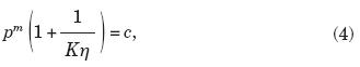
so that, since p^c = c,

Finally, our measure of welfare loss given in (3) can now be rewritten using (5) as

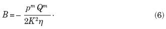
The appeal of this measure is evident: it just requires an estimate of the price elasticity, the spending on each good and the number of oligopolistic firms in the market (one in the case of a monopoly). Also note that one has to add the restriction η <–1/ K to equation (6), since it is needed for the optimality condition in (4) to hold.

 

II. Data and the Markets under Study

The household income and expenditure survey to be used here is known in Mexico as the Encuesta nacional de ingresos y gastos de los hogares, ENIGH, for short. The most recent ENIGH that was available at the moment of this writing was made in August-November 2006 (INEGI, 2007). The sample consisted of 20,875 housing units, and it was designed to provide reliable estimates at the national level, as well as at the urban and rural levels (the urban sector consists of all localities with 2,500 or more inhabitants, and the rural sector of the rest); furthermore, the 2006 survey was also representative for some, but not all, of the 32 Mexican states. For reasons to be given in a later section, it is important to add that the sampling process was stratified and multi-staged. Each primary sampling unit was made of one or several "basic geostatistical areas" (these are similar to the census tracts employed in other countries). The resulting 2,785 primary sampling units were subject to a stratification based on socio-demographic variables to finally produce 392 strata from which the sample was drawn.

Turning now to the markets to be studied, their selection is facilitated by the fact that soon after the survey was released the Federal Competition Commission listed a number of sectors that it wanted to examine closely (CFC, 2008). The goods mentioned by the Commission that are also included in the ENIGH are the following: corn tortilla, processed meats, carbonated soft drinks, cow milk, chicken and eggs, beer, medicines, electricity, liquefied gas, natural gas, and gasoline. On the other hand, the services included in that list that are also recorded in the survey are: foreign bus transportation, air transportation, private primary schools, private high schools, private universities, long-distance phone calls, local phone calls, cell phones, internet, medical fees, hospital fees, and credit card payments.

Even though all the goods and services mentioned above are reported in the ENIGH, for most of them there is only information on household spending, not on unit values. This is the case for both the services and the energy consumption goods. and services mentioned above are reported in the ENIGH, for most of them there is only information on household spending, not on unit values. This is the case for both the services and the energy consumption goods. Since this fact prevents us from a direct estimation of their corresponding price elasticities, in this paper we focus solely on the following seven consumption goods for which unit values are indeed reported: corn tortilla, processed meats (ham, bacon, sausage, etc.), carbonated soft drinks (together with juices and bottled water), cow milk, chicken and eggs, beer, and medicines (whether purchased with or without a prescription).

Having selected the goods markets, it remains to be decided whether or not each of them can be treated as a single national market. In our context, this would be so if there were no presumption of differing non-competitive practices across all regions in Mexico. Although in the case of urban areas there is no such presumption, in the case of rural areas there is evidence of distinctive non-competitive practices. For instance, it is common for firms to deliver directly their products to stores in remote areas, but only if no other competing brands are offered to the consumers. There are even documented cases (CFC, 1998) in which firms have bribed the leaders of communal lands to eject competitors from the entire locality. If we add to that evidence the fact that in most rural areas there are no shopping outlets nearby that can impose some price discipline, then it would seem important to distinguish between the urban and the rural sectors in what follows.

 

III. Price and Quality

Since the ENIGH is not a longitudinal survey, but rather a cross-sectional one, we should resist the temptation of treating the unit values reported by each household as the goods’ prices faced by the rest of them. This is so because variations in unit values across households may be due to changes in the quality of goods purchased; for instance, the price difference between two cuts of beef can be quite significant. Furthermore, even if the goods are identical, the perceived quality may differ; for example, the lettuce sold in a supermarket may be perceived to be cleaner than the one sold in a market street.

Although the above comments might be thought to imply that there is no way to estimate the own-price elasticities needed in this paper, there is however an indirect procedure that can be implemented for that end. The model of spatial variations due to Deaton (1988, 1990, 1997) can be used, provided that the unobserved prices do not vary within the clusters used in the sampling process. In the case of the ENIGH this is a reasonable assumption, since, as noted earlier, each of its 2,785 primary sampling units correspond to a simple geostatistical area, a neighborhood. Following the notation in Deaton (1997), the statistical model to be used is of the form:

where: M is the number of goods; w_Ghs is the share of good G in the budget of household h, located in the sampling unit (the cluster) s; x_hs is the household’s total spending; z_hs is a vector of socio-demographic variables (and ‘·’ is the inner product); π_Hs is the price of good H prevailing in the sampling unit s; f_Gs is a cluster-level effect (fixed or random) that is uncorrelated with the prices; ν_Ghs is the unit value of good G as reported by the household h, located in cluster s; and u_⁰Ghs and u_¹Ghs are the correlated stochastic residuals. There are S sampling units (clusters).

It is worth noting that the apparent similarity between the model (7)-(8) and the popular Almost Ideal Demand system is illusory. The model may be viewed, at best, as an aggregate demand system where "the averaging over agents almost never permits an interpretation in terms of a representative agent" (Deaton, 1997, p. 305). An implication of this fact is that, as already noted in section I, we cannot use in this paper utility-based measures to estimate welfare losses. Another consequence is that a special econometric procedure has to be used to estimate the model.

Since Deaton (1997, pp. 293-305) has a very detailed exposition of his methodology, here we limit ourselves to point out its main features. The estimation procedure can be divided into two parts. In the first, the within-cluster stage, the two equations (7)-(8) are run using ordinary least squares after demeaning, by their cluster means, the budget shares, the logarithms of the unit values and of the expenditures, and the socio-demographic variables. Since prices are constant in each cluster, then, as is well known from the literature, demeaning removes prices and fixed effects, and allows consistent estimation of the alphas, betas and gammas.

The second part, the between-cluster stage, is less canonical. As a first step, for each good G those consistent estimates of the parameters are used to compute the averages in each cluster s of, both, the shares and the log of the unit values, after purging them of the effects of expenditures and socio-demographic characteristics:

where n_s is the total number of households in the cluster (the sampling unit) s, and n_⁺Gs is the number of households that reported a unit value for the good. These averages are estimates of the following "true values" that would be obtained if one were to know the coefficients that multiply the own and cross prices of each good:

In the second step, the first-stage regressions are used to estimate not only the variance-covariance matrices of the vectors of the residuals in (7)-(8), corresponding to all clusters s, but also the variance-covariance matrices of the corresponding vectors of the theoretical averages given in (11)-(12). In particular, let Q and R be the estimators for the variance-covariance matrices of the vectors y¹_Gand u¹_G, and T and U the estimators for the covariance matrices of, respectively, y⁰_G and y¹_G, u⁰_G and u¹_G. For the purposes of finding the price-elasticity matrix, which is our main interest, define

where D(n⁺_s) is a diagonal matrix formed from the elements of n⁺_Gs, and likewise D(n_s) is a diagonal matrix formed from the elements of n_s. Also, consider the vectors and ζ with components _G and and define the corresponding diagonal matrices D() and D(ζ) formed from those components. Then, the price-elasticity matrix can finally be estimated as:

Having described the main lines of the estimation procedure, we now turn to our particular model. It is estimated for the seven goods under consideration after adding a number of socio-demographic variables. The first three of these last variables are the age of the head of the household, her years of education and the number of members of the household. The next ten variables are made of the following proportions: of men and women in the household that are under 12 years of age; of men and women aged 12 years or older, but under 25 years of age; of men and women aged 25 years or older, but under 45 years of age; of men and women aged 45 years or older, but under 65 years of age; and of men and women aged 65 years or older. Finally, binary variables were also included to capture diverse consumption patterns across regions. For that end, the 32 Mexican states were divided into four regions: Baja California, Baja California Sur, Coahuila, Chihuahua, Durango, Nuevo León, Sinaloa, Sonora and Tamaulipas; Aguascalientes, Colima, Guanajuato, Jalisco, Nayarit, San Luis Potosí and Zacatecas; Campeche, Chiapas, Guerrero, Oaxaca, Tabasco, Quintana Roo and Yucatán; and Distrito Federal, Hidalgo, Estado de México, Michoacán, Morelos, Puebla, Querétaro, Tlaxcala and Veracruz.

The estimation results, for both urban and rural households, are presented in table 1. As can be appreciated, the point estimates of the own-price elasticities seem to be reasonable in both sectors. Only the demand for milk is inelastic, at a level of significance of 5 per cent, for all households, while the demand for corn tortilla is also so for rural households (whose diet crucially depends on tortilla consumption). Although income elasticities are not included in the table, it may also be noted that only beer seems to be a luxury good in both sectors.¹

IV. Distributional and Regional Impacts

This part integrates the theoretical results developed in section I with the empirical results that have just been presented. As noted earlier, if for a given market we assume that firms produce a homogeneous product, have identical cost functions, and behave as in a Cournot-Nash game, then the corresponding welfare loss can be estimated using (6). However, in order to be able to establish comparisons across groups of individuals, it is convenient to re-scale each of those welfare losses as follows: given the notation in section III, let M be the number of goods purchased by the consumers from firms with market power. Then, a measure of the total welfare loss in relative terms can be found after dividing our defined welfare loss on each item by the total expenditure on the M goods:

where, as before, w_G is the share of good G in total expenditure, K_G is the number of firms in the market for that good, and η_G is the own-price elasticity of market demand. It is also worth remembering that the existence of an optimum requires that the elasticity itself is not only negative, but also that η_G < –1/ K_G (this condition collapses in the case of a monopoly to the classical condition that η_G < –1).

In order to compute (15) we have to specify the number of firms participating in each of the seven Cournot oligopolies. In the case of the market for corn tortilla, about half of its production is made after treating the corn kernels using an ancient technique called "nixtamalization", while the other half is made using corn flour. The first production process is practiced by myriads of small producers and households across the country, while 70 per cent of the supply of corn flour comes from a single company.² To represent that fact in our model we assume that those two inputs are perfect substitutes and that the firm faces a competition from the rest, so that K₁ = 2. It may be noted that, as implied by table 1, the necessary condition η₁ < –1/2 is not rejected at a 5 per cent level of significance in the case of both the urban and the rural sectors.

Turning now to the processed meat market, we assume that K₂ = 3 given that there are three companies relatively equal in size that clearly control it. Another three firms used to control the chicken and eggs markets until very recently, when imports have brought some price discipline. Yet, in 2006, when the ENIGH was made, K₃ = 3 would still seem to be the most adequate value. It may also be noted that, in the case of both processed meats and chicken and eggs, the corresponding condition η_i < –1/3 cannot be rejected.

In the case of milk, two companies control about 80 per cent of the market, while the other 20 per cent is geographically fragmented. Thus, for the simulation we take K₄ = 2 (note that the condition η₄ < –1/2 also cannot be rejected, although barely in the urban sector at a 5 per cent level of significance). Regarding soft drinks, there is a firm that controls about two thirds of the Mexican market, and it has also been fined twice by the Mexican Federal Competition Commission for monopolic practices. Thus, we set K₅ = 1, a value that is theoretically admissible since, as shown in table 1, the point estimates of the elasticities in both sectors are smaller than -1.

It would seem at first sight that the market for beer in Mexico constitutes the classical case of a duopoly, since there are only two producers. However, the market is segmented geographically and prices are curiously identical among competing brands (from light beer to dark beer). For many observers of the industry this is a case of conscious parallelism; that is, it is an instance of tacit price-fixing between the two competitors. Thus, we choose K₆ = 1 for the simulation below (a value that is admissible according to table 1). The final case, the market for medicines, is the most complex since there are several producers. Yet, except for the case of generic drugs, medicine prices in Mexico are considerably high according to international standards. Since the most favoured hypothesis to explain that phenomenon is once again conscious parallelism, we set K₇ = 1 (which is also admissible).

Using the values determined above, the own-price elasticities given in table 1 and the data on households’ income and spending, table 2 presents estimates of the distributive effects of market power. The results in the table are calculated after ordering, by deciles, urban or rural households according to their total monetary income (the lower the decile, the poorer the group). Next, using (15) we estimate for each household the relative welfare loss due to market power in the seven markets, and after that we compute an average of the losses among all households in each decile. Finally, those averages are expressed relative to the average of the decile that is affected the least by the market power of the firms.

The estimates thus obtained are presented in the second and fourth columns of table 2. The results suggest that in the urban sector the negative impact of monopoly power grows (in relative terms) as households become poorer. In the limit, the poorest households have a relative welfare loss about 19.8 per cent higher than the one suffered by the richest. For the rural sector the redistributive impact is even more serious, since the first decile has a relative welfare loss of about 26.4 per cent compared to the ninth decile, and of 22.7 per cent compared to the tenth decile.³

Given the substantial redistributive effects arising from monopoly power, one could also wonder about its regional impacts across the 32 Mexican states. This can be accomplished using a similar procedure as the one mentioned earlier, except that now urban and rural households are classified by their home states, not by their incomes. Map 1 illustrates the results thus obtained. The state with the smallest relative welfare loss turns out to be Baja California, which lies at the farthest north, while the state with the largest loss is Chiapas, at the farthest south. In fact, Chiapas’ relative welfare loss is 2.77 times larger than Baja California’s. More generally, the southern states, many of which are Mexico’s poorest, are those with the greatest welfare losses.

What factors might explain those results? There are essentially two: the percentage of households that live in the rural sector in the case of each state, as well as the very diverse consumption patterns that exist in Mexico. For instance, a majority of rural households live in the south, and for them the most important component of their diet is corn tortilla. As a final point, it should be recalled that the ENIGH is representative only for some states, so that our last results are less precise than the ones obtained earlier. Yet, we think that this last exercise is worth being presented, since a legislator would be even more concerned about the redistributive effects of market power if it just happened that her represented constituency were one of the most affected.

 

V. Other Approaches to Measure Welfare Losses

We do not want to conclude this paper without acknowledging that our methodology to measure the welfare loss due to monopoly power is only one of several possible approaches. To start with, one should note that the simple expression for welfare loss given in equation (6) rests on a key assumption: the net loss of consumers’ surplus can be used as an approximation for the welfare loss due to market power. Should that measure be replaced instead by the total loss of consumers’ surplus? That is, should we include in that welfare loss the profits made by the oligopolistic firms? The answer to that question depends on whether or not those excess profits are taxed and the corresponding revenue is later redistributed or not by the government. It is difficult to assure to what extent that is so in Mexico. But what is true is that the tax system that prevails in Mexico today is more progressive than one would thought at first sight: most households that are in the formal sector and are situated in the first four deciles, according to their total income, actually receive negative income taxes and also pay relatively small amounts of value added taxes (not only due to their low consumption, but also due to special vat regimes).Thus, it is not evident that one should count in the welfare losses the total amount of the firms’ excess profits; at least not in their entirety.

A second possible alternative to our approach has to do with our assumption, implicit in the linearization of the demand function to obtain expression (1),that elasticity changes as consumption changes. Another possibility could be to assume that the market demand is isoelastic: D(p)= ap^η , η < 0. However, although it can be shown that such a functional form leads to a Cournot-Nash equilibrium that depends only on the number of firms and the elasticity, it does so under two stringent assumptions: the welfare loss has to be equated to the total consumers’ loss, an assumption that we have criticized earlier, and the price elasticity has to be always the same, regardless of any variation in the unit values and the quality of the goods. This last supposition contrasts sharply with the highly complex expression for the elasticity matrix given in (14).

Still another possibility of estimating the welfare losses due to market power is by making use of data that is publicly available: the firms’ earnings before interest, taxes, depreciation and amortization (EBITDA). Although it does not include the cost of capital and the depreciation of long-life assets, and so it does not represent properly speaking economic profits, the EBIDTA could be used to approximate the so-called residual elasticity for each firm in a conjectural variations context (broader than our Cournot-Nash context). That is, after modifying equation (5) the EBIDTA could be used to estimate the left-hand side of

and the residual elasticity on the right-hand side could be estimated as well. This in turn could be used to infer the market elasticity (equal to K times the residual elasticity in our case).

The last alternative approach to be mentioned here contemplates the possibility of studying not only the goods markets for which a monopolist or oligopolistic behavior is presumed in Mexico, but also the corresponding markets for services. These later markets are also interesting to examine since, as opposed to the case of consumption goods, one would expect that the largest welfare losses due to market power would be suffered this time by the more affluent. Such an examination could be accomplished if one were willing to make two drastic assumptions: that the ENIGH could be treated as a longitudinal survey and that, following Frisch (1959), the underlying utility function could be deemed to be additive. Then, as illustrated in Urzúa (2009), one could obtain rough estimates of the price elasticities of services as well.

 

References

CFC (1998), "Actos tendientes a procurar la venta exclusiva de cervezas de marcas: Resolución SHP_RA-34-98", Mexico, Comisión Federal de Competencia, memo.         [ Links ]

---------- (2008), "Convocatoria para líderes de proyecto", Mexico, Comisión Federal de Competencia, memo.         [ Links ]

Comanor,W. S. and R. H. Smiley (1975),"Monopoly and the Distribution of Wealth", Quarterly Journal of Economics, 89 (2), pp. 177-194.         [ Links ]

Creedy, J. and R. Dixon (1998), "The Relative Burden of Monopoly on Households with Different Incomes", Economica, 65 (258), pp. 285-293.         [ Links ]

---------- (1999), "The Distributional Effects of Monopoly", Australian Economic Papers, 38 (3), pp. 223-237.         [ Links ]

Deaton, A. (1988), "Quality, Quantity and Spatial Variation of Price", American Economic Review, 78 (3), pp. 418-430.         [ Links ]

---------- (1990), "Price Elasticities from Survey Data: Extensions and Indonesian Results", Journal of Econometrics, 44 (3), pp. 281-309.         [ Links ]

---------- (1997), The Analysis of Household Surveys: A Microeconometric Approach to Development Policy, Washington, World Bank.         [ Links ]

Frisch, R. (1959),"A Complete Scheme for Computing All Direct and Cross Demand Elasticities in a Model with Many Sectors", Econometrica, 27 (2), pp. 177-196.         [ Links ]

Hausman, J. A. and J. G. Sidak (2004), "Why Do the Poor and the Less-Educated Pay More for Long-Distance Calls?", Contributions to Economic Analysis & Policy, 3 (1), pp. 1-26.         [ Links ]

INEGI (2007), Base de datos de la Encuesta Nacional de Ingresos y Gastos de los Hogares 2006, Aguascalientes, Instituto Nacional de Estadística y Geografía.         [ Links ]

McKenzie, G. (1983), Measuring Economic Welfare: New Methods, Cambridge, Cambridge University Press.         [ Links ]

Urzúa, C.M.(2009),"Efectos sobre el bienestar social de las empresas con poder de mercado en México", Finanzas Públicas, 1 (1), pp. 79-118.         [ Links ]

 

Notes

*The author thanks Francisco Rodríguez for his computational help, Ernesto Estrada and Pascual García-Alba for their helpful comments, and Ignacio Navarroand Javier Núñez for their suggestions.This paper is a reduced and modified version of an unpublished technical report, written in Spanish, which was prepared for the Mexican Federal Competition Commission. I am indebted to the Commission for financing the project, as well as for the comments of its reviewers. Last but not least, I am indebted to two anonymous referees for their very helpful suggestions. Needless to add, any opinions expressed in this paper are solely my own.

¹ Using the same ordering as in the table, the income elasticities are estimated to be 0.467, 0.498, 0.365, 0.639, 0.687, 2.107 and 0.606 for the urban sector, and 0.648, 0.761, 0.440, 0.769, 0.729, 2.019 and 0.835 for the rural sector.

² Since the names of the firms that have market power are irrelevant for the purposes of this paper, they have been entirely omitted. Nevertheless, they are available from the author upon request.

³As one would expect, the bootstrapped standard errors for the estimates in both columns turn out to be larger in the case of the rural sector. Furthermore, the null hypothesis that the relative welfare loss of rural households in the ninth decile is greater than the ones in the tenth decile can be rejected at a 5 per cent level of significance.