


Serviços Personalizados
Journal
Artigo
 Inglês (pdf)
 Artigo em XML
 Referências do artigo
 Enviar este artigo por email
Indicadores
-
 Citado por SciELO
 -
 Acessos
Links relacionados
-
 Similares em
SciELO
Similares em
SciELO
Compartilhar

 Permalink
Economía mexicana. Nueva época
versão impressa ISSN 1665-2045
Econ. mex. Nueva época vol.22 no.2 Ciudad de México Jan. 2013
Artículos
Why Did Wage Inequality Decrease in Mexico after NAFTA?
¿Por qué se redujo la desigualdad salarial en México después del TLCAN?
Raymundo M. Campos-Vázquez
Professor and researcher, Centro de Estudios Económicos, Colmex, Mexico City. rmcampos@colmex.mx
Fecha de recepción: 31 de enero de 2011;
fecha de aceptación: 7 de noviembre de 2011.
Abstract
Contrary to what happened before NAFTA, wage inequality in Mexico decreased after 1994. This paper investigates the forces behind the post-NAFTA decrease in wage inequality. Using a quantile decomposition, I show that the decline in wage inequality is driven by a decline in the returns to education and potential experience, especially at the top of the wage distribution. Supply and demand are the main contributors to this change. On the supply side, there were substantial increases in college enrollment rates after 1994, which translated into an increase in the proportion of workers with a college degree. However, this increase in supply was not met by an increase in demand for the highly educated: the proportion of the workforce in top qualified occupations and close to the top occupations did not increase as much as the increase in supply. As a result, college educated workers exercised wage pressure in top and less-than-top qualified occupations. A Bound and Johnson (1992) decomposition confirms that changes in relative supply are the main determinant behind the decrease in wage inequality.
Keywords: wage inequality, Mexico, education, employment.
Resumen
Contrario a lo que ocurrió con el TLCAN, la desigualdad salarial en México disminuyó después de 1994. Este artículo investiga las fuerzas detrás de la caída en desigualdad en el periodo posterior al TLCAN. Por medio de una descomposición cuantil muestro que la caída en desigualdad se deriva de una caída en los retornos a la educación y experiencia, especialmente en la parte alta de la distribución de salario. Oferta y demanda son las causantes de ese cambio. Por el lado de la oferta existieron aumentos sustanciales en la tasa de matriculación de la educación superior después de 1994, lo que se tradujo en un incremento en la proporción de trabajadores con esa educación. Sin embargo, este incremento de oferta no coincidió con un incremento en la demanda por esos trabajadores: la proporción de trabajadores en ocupaciones de alto salario no se incrementó tanto como la oferta. Como resultado, los trabajadores con educación superior pusieron presión salarial en ocupaciones con ingreso medio-alto y alto. Se aplica la descomposición de Bound y Johnson (1992) y se confirma que aumentos en la oferta relativa son el determinante principal detrás de la caída en la desigualdad salarial.
Palabras clave: desigualdad salarial, México, educación, empleo.
JEL classification: J20, J31, O15,O54.
Introduction
Inequality, measured using either income or wages, is an important topic that has been continuously debated among academics and the media. Since the 1980s, most countries in the world experienced an increase in wage inequality, and for some countries this trend continued during the 1990s. Mexico was no exception and went through a period of increasing inequality by the end of the 1980s. However, wage inequality in Mexico started to decline after 1994, the period after NAFTA was enacted. This could be surprising, given the relatively large literature explaining the causes of the increase in inequality in the late 1980s and early 1990s.1 Figure 1 documents the patterns of wage inequality in Mexico. Even though the decline has been taking place since 1994-1996, there are few references for this episode in the literature.2 In this paper I try to fill this gap and I give an explanation for the potential causes of this episode.

Wage inequality has continuously increased during the last 20 years in the United States and other developed countries (Katz and Autor, 1999, table 10). There is a debate about the causes of this increase. On the one hand, David Autor, Lawrence Katz and Daron Acemoglu among others (Acemoglu, 2002; Autor, Levy and Murnane, 2003; Autor et al., 2005, 2007, 2008) argue that skill biased technical change is the leading explanation for the increase in wage inequality. Since the supply of college educated workers increased during the period, the only possible explanation is that demand increased more than supply, and that the growth in demand is biased toward skilled workers. On the other hand, Thomas Lemieux, David Card and John Dinardo among others (Card and DiNardo, 2002; DiNardo, Fortin and Lemieux, 1996; Lemieux, 2006, 2008), criticize the view of skill biased technical change as the main source for changes in wage inequality. Instead, they argue that the increase in wage inequality at the end of the 1980s and beginning of 1990s can be seen as an episodic event rather than driven by skill biased technical change. According to their estimates, most of the increase in wage inequality, especially at the bottom of the wage distribution in that period, can be explained by the fall in the real minimum wage and a decline in unionization rates. More recently, Autor, Katz and Kearney (2008) recognize changes in the real value of the minimum wage and the fall of unionization rates as plausible explanations for the changes in lower tail inequality. However, they point out that institutional aspects cannot explain the continuous rise in upper tail inequality. They conclude that the increase in upper tail inequality cannot be explained by quantities but by returns, justifying the view of skill biased technical change as an important source for changes in wage inequality.
In some developed countries the wage structure has been changing favoring the high and low skilled workers. This process increases upper tail wage inequality but reduces lower tail inequality. For the U.S., Autor, Katz and Kearney (2007) show how high skilled jobs (occupations) in 1980 were the ones with the highest increase in demand, measured by the increase in the proportion of workers in those occupations. They also find that occupations in the lower tail increased their participation in the workforce, though at the expense of middle-tier jobs. Furthermore, in the U.K. Goos and Maning (2007) find a similar pattern to that in the U.S., and call this U-shaped pattern "job polarization". They conclude that skill biased technical change and job polarization are plausible explanations for the increase in wage inequality. In Germany, Dustmann, Ludsteck and Schonberg (2009) and Spitz-Oener (2006) find that job polarization is present, and that the increase in wage inequality can be explained in part by that process.
As explained above, inequality has continuously grown in developed countries since the 1980s. In contrast, Mexico exhibits a decrease in inequality after 1994. In this paper I explore the causes of such a decline. This is important for at least three reasons. First, societies generally prefer a more egalitarian distribution of resources. Hence, the example of Mexico may be useful to similar countries that desire to attain lower inequality levels. Second, it is also interesting to investigate whether Mexico has "job polarized" as other countries have, and analyze how this process modifies the wage distribution. Finally, other Latin American countries have recently experienced a decline in wage inequality; hence, the Mexican experience could help in building a consensus on why wage inequality has fallen in the region.3
In order to analyze the sources of the fall in wage inequality, I follow the Machado and Mata (2005) decomposition. In particular, I estimate quantile regressions and build counterfactuals of the wage distribution holding constant observable characteristics or returns in schooling and potential labor experience. This decomposition is similar to the DiNardo, Fortin and Lemieux (1996) non-parametric decomposition. The goal is to estimate the level of inequality using the endowments from one specific year, but assuming return values for a different year and vice versa. The results of the decomposition show that the returns to education and labor experience are the most important factor explaining the decrease in wage inequality. The decline in returns is explained by a substantial increase in college graduates in the last 10 years, but it is also due to slower growth in labor demand, especially for the top paid jobs. I divide jobs by "quality" using the occupation median wage in 1992, and show that top quality jobs did not grow as much as the increase in supply of high-skilled workers. Instead, low wage jobs increased their participation substantially at the expense of jobs in the middle of the distribution. In order to present further evidence on the effects of supply and demand, I decompose relative wage changes as in Bound and Johnson (1992). These results confirm that changes in relative supply are the main determinant behind the decrease in wage inequality.
A few recent papers have discussed the issue of why inequality in Mexico has fallen since NAFTA. Esquivel (2009) argues that the fall in inequality could be explained by a change in the composition of workers, and as a late outcome of trade liberalization. Robertson (2004, 2007) states that the fall in wage inequality is driven by traditional trade channels. Furthermore, Robertson (2007) asserts that workers in Mexico since NAFTA appeared to be complements to U.S. workers, not substitutes. López-Acevedo (2006), using data for the period 1996-2002, shows how a different education composition structure affects earnings inequality. The current paper differentiates from the previous ones in several ways. First, this paper explores competing explanations of changes in wage inequality. Second, it provides empirical evidence on the job polarization hypothesis, a theory that has not previously been tested in Mexico. Finally, it formally decomposes the effect of returns and endowments of the labor force on the wage structure in Mexico. Using these decompositions, one can create counter-factuals of what would have happened to the wage distribution had the returns or endowments been constant throughout the period. Previous papers do not attempt to construct counterfactuals.
The paper is structured as follows. In the first section I describe the basic facts and trends of wage inequality in Mexico for different groups. Then I contrast different hypotheses of the decline of wage inequality in the last years. The third section introduces the Machado and Mata (2005) methodology in order to decompose wage inequality. In this section I present results for this decomposition, analyze whether job polarization occurred in Mexico, and relate this process to the change in wage inequality. I then calculate the per cent effect driven by supply, and the one driven by demand factors, following the Bound and Johnson (1992) decomposition. The fifth and final section offers some concluding remarks.
I. Facts
There are three sources of data in Mexico that can be used to calculate wage inequality: Expenditure Survey, Labor Survey and the Population Census. Census data is not used because there are only two points in time (1990 and 2000), and most of the decline in wage inequality is for the period 1998-2006. The labor survey has two drawbacks: it is not nationally representative given that it only has data for urban areas and, more importantly, its methodology changed after 2004 rendering it useless for my purposes. For those reasons, my analysis will be based on the Expenditure survey (ENIGH). The ENIGH is nationally representative and includes relevant variables such as income sources, expenditures and demographic characteristics. ENIGH surveys can be compared across years. ENIGH is available every two years since 1992, plus years 1989 and 2005.4
In what follows I restrict the sample to all 18-65 year old workers with positive working hours and valid wage. When calculating hourly wage I follow Airola and Juhn (2005), and calculate monthly wage over 4.33 times hours of work, and when calculating descriptive statistics I use, as a weight, the person weight from the data times hours of work, as is commonly used in the wage inequality literature. Wages are in constant 2006 Mexican Pesos (MXP). I drop observations with real hourly wage less than $1 MXP.5,6
Figure 1 Panel A plots the trends of wage inequality in Mexico since 1989 using the log difference between the 90th and 10th percentiles. As has been documented in the literature, Mexico experienced a large increase in wage inequality in the period before 1994. What has not been documented equally widely is the substantial decrease in wage inequality after 1994. This decline applies to both males and females, although the decline is more consistent for males. Wage inequality has decreased by more than 20 log points during this period. Panels B and C decompose wage inequality using the log difference between the 90th and 50th and the 50th and 10th percentiles respectively. Panel B shows a decline in top wage inequality, while Panel C shows a decline in bottom wage inequality, although not as strong as the decline in top wage inequality.
Figure 1 exhibits a decline in wage inequality mainly driven by individuals in the top of the wage distribution.7 In order to analyze more carefully the change in wage inequality during 1994-2006, figure 2 Panel A presents the change in the log wage by centiles of the wage distribution using years 1994 and 2006.8 For example, the first decile (up to quantile 10) experienced an increase in real wages close to 5 per cent between 1994 and 2006. This graph indicates that there was an increase in the real wage of workers at the bottom half of the wage distribution. In fact, percentiles in the top half experienced a decrease in real wages, and this decline was even larger for top percentiles (although again, for women, this is not the case). The real wage of the top decile decreased on average 30 per cent.

The Mexican Peso crisis at the end of 1994 cannot explain the full decline in wage inequality during this period.9 For example, Panel B uses years 1996 and 2006 and shows that real wages at the top are still declining in comparison to different wages across the wage distribution, especially those at the very top.10 Deciles 2-4 had the highest wage increases during the whole period.
Finally, Panel C plots the change in wage inequality for years 19892006. Wages for the bottom half of the distribution (males and females) were more or less constant, with substantial increases for the very poor. The real losers in this period were those individuals in the "middle-class" and some high earners. Wages for workers between the 50th and 80th percentile decreased by approximately 5 per cent on average. Wages for workers between the 80th and 90th percentile decreased by approximately 3 per cent on average. The top decile increased their wages by roughly 6 per cent on average. Also, females substantially improved their wages at the top of the distribution. The key point in figure 2 is that the evolution of wage inequality in Mexico needs to be separated before and after NAFTA.
In sum, figures 1 and 2 demonstrate that something affected the Mexican economy during the period 1994-2006, causing a decline in wage inequality. Table 1 analyzes this issue more carefully and presents information on how real wages have evolved for different groups of workers. I follow Autor, Katz and Kearney (2008) and analyze subgroups of workers divided by gender, education (less than secondary, secondary, high school and college), and potential experience (1-20 years of experience and more than 20 years of experience) for a total of 16 groups.11 Then I calculate mean wages for each group and the proportion of workers in that group.

Table 1 shows the decline in real hourly wages after the Mexican Peso crisis of 1994. However, in general there was a strong recovery during the period 1996-2000. After 2000, wages have been stagnant. The wages of workers with less than a high school degree increased the most for the period after NAFTA (1996-2006), especially for males. Looking at the education groups, it is surprising that the wages of workers with a high school degree and those with a college degree have gone down after 2000 for both experience groups. At the same time, we can notice that there was an increase in the proportion of workers with high school and college degrees during the period 1989-2006, especially for women. For example, the proportion of female workers with a college degree with less than 20 years of experience increased 2.6 percentage points, and for females with a high school degree the increment was 2.7 percentage points.
Table 1 gives us an idea that there is a striking difference in terms of the proportion of workers with different educational levels. The proportion of female workers with secondary education increased by 1 percentage point between 1989 and 1996 for both experience groups, but it declined between 1996 and 2006 for the group with less than 20 years of experience. In contrast, although male and female workers with high school (adding experience groups) increased their participation approximately by 1 percentage point in the period 1989-1996, their participation in the workforce grew 2.1 and 4 percentage points for males and females respectively in the period 1996-2006. A similar pattern can be depicted for college workers. In sum, table 1 points out a difference in the proportion of workers in different education groups between the 1989-1996 and 1996-2006 periods.
II. Hypothesis
Following the seminal work by Bound and Johnson (1992) and the literature reviewed in Machin (2008), we can distinguish two forces that affect the wage structure. First, competitive factors such as the change in supply and demand of workers affect directly the wages of those workers. Second, non-competitive factors such as changes in minimum wages and unionization rates may explain variations in the wage structure. The main hypothesis in the current paper is that changes in the wage structure in Mexico for the post-NAFTA period are driven primarily by supply and demand forces.
There are many papers analyzing the role of unions and minimum wage on inequality in Mexico for the period before 1996. Fairris (2003) and Fairris and Levine (2003) conclude that the falling unionization rate between 1984 and 1996 explains 11 per cent of the increase in wage inequality. Kaplan and Novaro (2006) and Bosch and Manacorda (2010) analyze the effect of the minimum wage on the wage structure and wage inequality during the 1989-1994 period and later years. In particular, Kaplan and Novaro (2006) argue that although the minimum wage is not binding in Mexico, it affects other wages in the distribution (a similar result is provided by Fairris, Popli and Zepeda, 2008). Bosch and Manacorda (2010) argue that the increase in wage inequality for the period 1989-2000 can be explained by a falling real minimum wage, especially for the period 1989-1996.12
If institutional factors were fundamentally altered during the post NAFTA period, then those changes could explain variations in the wage structure. However, unionization rates and the real minimum wage have been constant throughout the period in Mexico, and, as a consequence, they are unable to explain the decline in wage inequality. Moreover, institutions cannot explain the decline in top wage inequality. Figure 3 depicts the trends of the unionization rate and the real minimum wage for the period 1989-2006. Before 1994 there is a sharp decline in both the unionization rate and the minimum wage. The unionization rate fell almost 6 percentage points during 1989-2006, and the minimum wage lost 30 per cent of its real value. However, for the period 1996-2006 both the unionization rate and the real minimum wage were fairly constant. The real value of the minimum wage practically did not suffer any changes, while the unionization rate fell by 2 percentage points, although this fall was mainly driven by the year 2006.

Since institutional factors were not significantly altered during the period 1996-2006, the causes of the decline in wage inequality, especially at the top, need to be found elsewhere. It is possible that a constant minimum wage helped to keep constant lower tail inequality, but it is hard to argue that a constant minimum wage caused a decline in top wage inequality.
As for the competitive factors on the demand side, two leading (and confounding) forces driving wage inequality have been raised: trade and skill biased technical change.13 Cragg and Epelbaum (1996) and Esquivel and Rodríguez-López (2003) argue that most of the increase in wage inequality before NAFTA is driven by skill biased technical change. Given that trade liberalization in Mexico occurred in the mid-1980s, the Stolper-Samuelson theorem would have predicted a decrease in wage inequality, not an increase. In particular, Cragg and Epelbaum (1996) conclude that the trade sector in the economy became more skill-intensive, suggesting a decline in demand for less skilled workers. Robertson (2004, 2007) analyzes the role of trade for the period after NAFTA. He mentions that trade caused a reorientation of Mexican manufacturing benefiting less skilled workers.14
However, empirical applications face a serious challenge in separating the effects of trade, skill biased technical change and other changes in demand when using samples for the full population. For example, Esquivel (2009) finds that wage inequality decreased among all industries (not only manufacturing) and regions.15 Hence, trade theories need to explain why trade affects all industries in a similar way. Moreover, some studies restrict their analysis to the manufacturing industry in order to identify the trade effect, but the proportion of manufacturing workers is round 20 per cent, and not representative of all workers. Given these criticisms, instead of separating each demand effect on wages, I calculate changes in total demand as in Bound and Johnson (1992) and Goos and Manning (2007).
Following the Bound and Johnson (1992) decomposition, I argue that there are two main reasons for the decline in wage inequality. The first reason is the substantial increase in schooling after 1990, especially in the second half of the 1990s after the 1992 reform, which imposed mandatory secondary education. The second reason involves an absence of top quality jobs creation or a lack of growth in labor demand for skilled workers.
Figure 4 plots enrollment rates adjusted for population since 1980.16 Before 1994 there is no substantial increase in enrollment rates. High school education attendance increased slightly but this increment is mainly driven by the increase during 1980-1985, and after 1985 enrollment did not increase. College enrollment was fairly constant during the 1980-1994 period. The supply of skilled workers did not change substantially for the period before 1994 (see table 1). The main goal of figure 4 is to show a clear change in enrollment rates after 1994. Hence, the figure shows that the increase in higher educated workers (table 1) comes from a higher attendance rate.
Figure 5 plots the relative wage and relative supply of workers with at most secondary education and college education in log levels. The first y-axis includes the log of the ratio of wage between secondary and college educated workers. The second y-axis includes the proportion of workers in the same education categories. Both wages and proportion of workers are obtained from the estimates provided in table 1. The trend in the proportion of workers has been smoothed using a simple moving average; I multiply the previous and post period by 0.25 respectively and add the current period times 0.50. Before 1994, the trends cannot be related to each other. After 1996, and especially after 2000 inclusive, the trends between wages and proportion of workers are negatively correlated. The timing of the decline in relative wages coincides with the expansion of enrollment rates for college education shown in figure 4 (adding the four years of college education).

Assuming that other factors like demand and skill biased technical change are negligible, figure 5 implies that the elasticity of substitution between secondary and college workers is above unity (for the 1996-2006 period).17 This elasticity implies that, holding other factors constant, a decrease in the proportion of workers with secondary education relative to the share of those with college education by one per cent raises the relative wage by slightly less than one per cent. Section IV, below, analyzes changes in relative supply and their effect in relative wages for different elasticities of substitution.
Although the change in educational levels is an important factor to explain the decrease in wage inequality, it cannot be the only explanation. If college education increases and the returns to college are unchanged, then inequality has to increase given the small proportion of workers with college education. Hence, returns to college education are lower now than they were in 1994. A decrease in demand for college educated workers explains also part of the decline in the returns to college. Even though the decline in wage inequality can be seen as something positive for society, it is not an entirely good thing given that recent college graduates have not been able to find high quality jobs. In particular, college educated workers have been downgraded in occupational terms and are putting pressure to workers in lower occupational skills. Labor demand and job creation have not been able to absorb all the increase in the supply of skilled workers. The next section analyzes more carefully both claims.
III. Results
Quantile decomposition
In this subsection I analyze the effects of the increase in educational levels on wage inequality, using the Machado and Mata (2005) decomposition. This decomposition analyzes whether changes in wage inequality are driven mainly by quantities (endowments) or by prices (returns), as in the Oaxaca-Blinder decomposition or in the non-parametric decomposition suggested by DiNardo, Fortin and Lemieux (1996). The only difference here is that, instead of using the means only, the decomposition uses quantiles of the full wage distribution. The conditions for this procedure to work are that the characterization of the quantile regressions needs to be correctly specified, that quantile regression estimates are accurate predictors of the true wage distribution, and finally the assumption of partial equilibrium. The last assumption means that if returns are increasing, individuals do not increase their levels of schooling because of the rise in returns.
The implementation is straightforward. First, I estimate conditional quantile regressions separately for each year and gender; I estimate regressions for quantiles θ = 0.01,0.02,...,0.99. I follow Autor, Katz and Kearney (2005) and estimate a flexible functional form based on education and potential experience.18 Second, I save the coefficients for each quantile and year. Third, I calculate counterfactuals based on the endowment distribution for one year using the returns of a different year. For example, to calculate the change in inequality in quantile θ caused by changes in quantities between year t and τ using the returns as in year τ, we calculate:
Qθ( Xτßτ) - Qθ(Xt ßτ)
where Qθ (.) is the result of multiplying the vector of parameters to each observation in the dataset, and θ represents the quantile of the resulting distribution.19 Notice that in the decomposition one can assume the returns to be those of year τ, but it is also possible to set them to be those of year t. Hence, Qθ( Xτßτ) - Qθ(Xt ßτ) is the change in wage inequality explained by the change in endowments, assuming prices to be those of year τ. Like the Oaxaca-Blinder decomposition, the total observed change in inequality can be decomposed as
(Qθ( Xτßτ) - Qθ(Xt ßτ)) + (Qθ( Xτßτ) - Qθ(Xt ßt)) + ε
where the first term is the estimated effect of quantities or endowments, the second is the effect of prices or returns, and the last one is the residual. Obviously, the effects of quantities and prices are determined by what factor is taken into account first. In the calculations below I change the order of the decomposition to check the robustness of the results. Also, we expect the residual to be close to zero, that is, we expect the quantile estimation to be very close to the actual distribution; otherwise, it is possible that decomposing wage inequality with quantiles is not valid.20
Table 2 shows the main results of this decomposition. This table includes the quantile decomposition for three different periods: 1996-2006, 1994-2006 and 1989-2006. Each period includes the observed change in wage inequality, the effect due to quantities and prices, and the residual. In the first row I decompose wage inequality using quantities first and then prices for each group. The second row for each group (in italics) includes the decomposition in the reverse order: prices first and then quantities. The main results are those for the period 1996-2006, and the rest of the periods is used as a robustness check and to compare the results with those from previous literature. For males, using the wage differential 9010, the observed change in wage inequality for the period 1996-2006 was -0.10. Had returns been constant, wage inequality would have increased 0.17-0.23. On the other hand, had endowments been constant wage inequality would have fallen approximately to 0.3.
The change in wage inequality in the top half of the wage distribution can be mostly explained by a change in returns for the periods 1994-2006 and 1996-2006. The order of the decomposition does not matter, suggesting that prices are an important determinant of the decline in wage inequality. Given the 1994 economic crisis, the decomposition works better for the period 1996-2006 than for the period 1994-2006. The residual is larger for the latter case. On the other hand, the decomposition for the period 1989-2006 works poorly as the sign of the estimates changes according to the order of the decomposition. This suggests that the economic crisis is an important factor and that there are non-competitive factors affecting the wage distribution. Factors such as unionization, real minimum wages and industry rents are important factors that affected the wage distribution during the period 1989-1994.21 Bosch and Manacorda (2010) argue that most of the increase in wage inequality between 1989 and 2000, especially at the bottom of the distribution, can be explained by a declining real minimum wage. This is consistent with the quantile decomposition, given the large residuals found for the period 1989-1994 and the inability of the model to predict correctly the change in inequality at the bottom of the distribution.
Results in table 2 show that the decrease in wage inequality is mainly driven by a fall in the returns to schooling. Given the low levels of schooling in Mexico, if returns to education had been constant then an increase in schooling would have increased (not decreased) wage inequality. This is true for males and females, except in the case of top wage inequality for females.22 For the period 1996-2006 the order of the decomposition does not matter; the results are closely similar. The decomposition works better for the wage differential 90-10 and 90-50 than for the 50-10. Inequality at the bottom almost did not change, so the decomposition does not do a very good job. The effect of prices is concentrated at the top-half of the distribution.23 In sum, the results show that had returns kept constant, inequality would have increased. Hence, the fall in inequality is driven by a fall in returns to education, which is caused by a higher relative supply in college educated workers.
III.2. Job polarization and Demand of High Quality Jobs
The second reason why inequality has fallen is the lack of creation of high quality jobs. In the last 20 years, developed countries have experienced a process known as "job polarization." Studies for the U.S., England and Germany provide evidence that the increase in wage inequality in these countries is driven by an increase in top wage inequality (Autor, Katz, and Kearney, 2007; Goos and Manning, 2007; and Dustmann, Ludsteck, and Schonberg, 2009). In particular, these studies find that labor demand for top qualified occupations (ranked by wage paid in a previous year) has increased. At the same time, as low qualified occupations are likely complements to top qualified occupations, demand for low paid occupations has increased and demand for middle paid occupations has decreased. This process leads to a decrease in bottom wage inequality but to an increase in top wage inequality.
If the demand in Mexico for top qualified jobs is growing, one can expect the supply of workers with college education to be absorbed by those jobs. If the labor demand growth rate is constant or increasing for the period 19962006, the proportion of workers in top qualified occupations should increase. Following Goos and Manning (2007), a simple way to show this is creating a graph in which the x-axis reflects the rankings of occupations (measured by the median wage) and the y-axis reflects the change in the proportion of workers in those occupations during the specified period.
I rank occupations based on the median wage of 1992 and then collapse them according to deciles.24 Then I calculate the proportion of workers (hours adjusted) in each decile and the change in the proportion of workers for different periods. Figure 6 Panel A presents the plot for the periods 1994-2006 and 1996-2006. Demand for the lowest paid occupation (agricultural workers) fell the most during both periods. However, low-paid occupations in deciles 2-4 increased their participation in the workforce, and at the same time high-paid occupations did not increase their participation as much as low-paid occupations did.

The increase in the proportion of workers in top qualified jobs was less than 1 percentage point between 1996-2006. The largest declines in this period besides agricultural jobs are found close to top qualified occupations, like secretaries, some workers in manufacturing and some technicians in social sciences and medicine. As shown above, the 1996-2006 period experienced large increases in high school and college education, but these workers were not absorbed by the top qualified jobs.
Among the highest increase in demand for low paid occupations are the following: in decile 2, construction workers and domestic service workers; decile 3, food, drinks and tobacco manufacturing workers and waiters; decile 4, employees in retail trade and textile workers. For the top two deciles, the main occupations that experienced demand growth are those corresponding to professionals in the social sciences; however, many professional occupations did not experience an increase in demand. Tables 3 and 4 analyze the occupations in the bottom and top half of the wage distribution of 1992, and include the mean wage for some occupations as well as the proportion of workers in that occupation for different years. The largest increment in employment was given by employees in retail trade.


Autor, Levy and Murnane (2003) argue that computers are the causal mechanism of job polarization. As prices of computers decline, demand for occupations in which workers are complements to computers increases causing a rise in the wage paid to those occupations. However, at the same time the demand for other occupations in which workers are substitutes to computers declines. Since computers are substitutes for workers in occupations that are in the middle of the distribution, the decrease in the demand for middle-tier jobs causes an increase in wage inequality at the top of the distribution. In Mexico, some job polarization process is observed. Demand for workers in occupations that are close substitutes to computers declined: secretaries, some workers in manufacturing, technicians. However, demand for workers in occupations that are complements to computers did not increase. In the last row of table 4 I include the mean wage for all professional workers and business managers and directors, as well as the proportion of workers in those occupations. It is striking that the proportion of workers in those occupations did not increase substantially. Between 1996 and 2006 the proportion of workers increased by only 0.72 percentage points.
As the share of workers with college education rised 5 percentage points in 1996-2006 (table 1), we would expect similar increases in professional occupations. But the main professional occupations (social sciences, economics, accounting and engineering) increased their participation in less than one percentage point, as table 4 suggests. College educated workers needed to downgrade, in order to work, for lower paid occupations. Figure 6 Panel B calculates the change in the share of workers with college degree within each decile. This graph shows that deciles 8-10 had the largest increments in college educated workers. Since the demand in top decile occupations could not absorb the supply of college graduates, college educated workers had to downgrade to lower paid occupations.
The results shown in this section depict a story where demand has not been growing enough to keep up with the substantial increase in supply, especially for college educated workers. Job polarization is present in the bottom half of the occupations, but there is no substantial increase in demand in the top paid occupations. The excess supply of workers with college degree creates wage pressures not only in top quality jobs, but also in less-than-top quality jobs. As the enrollment rates for college individuals continue to grow, this process will probably put more pressure on wages at the top of the distribution.
IV. Bound and Johnson (1992) Decomposition
In order to examine the effect of supply and demand on relative wages, I follow the Bound and Johnson (1992) decomposition and apply it to the case of Mexico for the period 1996-2006. I further assume that non-competitive sources are not important during this period and then determine the relative importance of supply and demand factors. Assuming a simple CES production function with elasticity of substitution, σ, constant across skills, it is possible to determine the effect of supply and demand on relative wages. In particular, it is possible to show that the relative wage of workers with college degree in terms of the wage of workers with at most secondary education can be expressed in terms of its increase in demand and supply:

The residual term ξ contains the effect of skill biased technical change and other non-competitive factors. As the unionization rate and the real minimum wage were fairly constant during 1996-2006, I assume non-competitive factors are negligible. The supply component is easily calculated from table 1 and refers to the relative increase of college educated workers over secondary educated workers.25 I follow Bound and Johnson (1992) to calculate the increase in relative demand. I construct the index as:
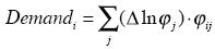
where φj is the proportion of workers in industry j, and φij is the proportion of workers of group i in industry j.26 In order to calculate the per cent change of demand for college educated workers over secondary educated workers, I take the difference between the predicted increase in demand for college workers and secondary educated workers, DemandCollege - DemandSecondary.
Table 5 includes the decomposition of relative wage changes between college educated workers and secondary educated workers. Figure 5 and table 1 show that, for males, college educated workers' wage relative to secondary educated workers' declined 20 log points between 1996 and 2006. The relative supply, on the other hand, rised 27 log points during the same period. If the elasticity of substitution is assumed to be equal to 2, then relative supply changes explained 100 per cent of the reduction in wages for all workers, and 63 per cent of the decline in males' wages. The calculated demand components are small in magnitude but negative, suggesting that relative demand between college and secondary educated workers actually dropped. This result is consistent with the findings in the previous section and with what is shown in figure 6. After NAFTA, labor demand did not increase for high skilled workers. The residuals for the full sample as well as for men only, in table 5, are relatively small. The small residual suggests that skill biased technical change was not important during this period, in contrast to findings for the 1989-1996 period (see Esquivel and Rodríguez-López, 2003).

Autor, Levy and Murnane (2003) argue that the causal mechanism for skill biased technical change is the price of computers. As the price of computers declines, demand for jobs in which workers are complements to computers increases. Previous research on wage inequality in Mexico before NAFTA has suggested that skill biased technical change is one of the main reasons why wage inequality increased during this period.27 However, table 5 implies that skill biased technical change is relatively unimportant given the small residual after NAFTA. In fact, as computer prices have been decreasing during the last 20 years, this implies that skill biased technical change may have a less significant role before NAFTA than previously though.
V. Conclusions
As opposed to many developed countries, wage inequality in Mexico has been falling for the period after 1994. This decreasing trend is mainly driven by supply and demand forces. Institutional factors such as the unionization rate and the real minimum wage did not adjust significantly during this period and hence they cannot explain the substantial decrease in wage inequality at the top of the wage distribution. Enrollment rates in Mexico were fairly constant for the period 1980-1994. Only after 1994 did Mexico substantially increase its enrollment rates of college and high school. This rise in educational attainment caused a decline in wage inequality after 1996 through a decrease in returns to education. The second reason of the fall in inequality is a slower demand growth. In particular, the increase in supply of college educated workers was not matched by an increment in top qualified jobs.
Job polarization in Mexico is different from the one experienced in other countries. Although the proportion of workers in "lousy jobs", as defined by Goos and Manning (2007), is increasing, the "lovely jobs" do not show a corresponding rise in the proportion of workers. The slow growth in top paid occupations is surprising considering the increase in demand for them in the U.S. and the U.K. More research is needed not only to know how computers increase labor demand for top paid occupations, but also to check whether there are fixed costs in the adoption of new technologies and what institutional factors are preventing the labor demand from growing through the use of computers in Mexico.
The Bound and Johnson (1992) decomposition suggests that increments in the supply of college educated workers are the main source of the reduction in wage inequality. The decomposition also implies that a lack of job creation is responsible, too, for the lower wage inequality that Mexico experienced after NAFTA. These two mechanisms imply that skill biased technical change did not play a substantial role in the modification of wage distribution. Moreover, if the price of computers decreased more in the period after NAFTA than it did before its enactment, and computers are the causal mechanism for skill biased technical change, the results in this paper cast caution on the explanation that skill biased technical change was the reason behind the rise of wage inequality before NAFTA. Moreover, results in this paper are consistent with other findings in Latin America, as reviewed in Lopez-Calva and Lustig (2009). The increase in the relative supply of skilled workers has altered the relative returns of those workers. Moreover, changes in demand have not offset the increase in the supply of skilled workers.
Lower wage inequality can be a desirable goal for any society. However, Mexico has experienced lower wage inequality partially for not being able to create enough top quality jobs. In sum, the demand for college educated workers did not grow as much as the supply. This process caused wage pressures for top quality jobs and for less-than-top quality jobs, resulting in lower wage inequality.
The experience of Mexico can be interesting for other developing countries. On the one hand, it is possible to reduce wage inequality with substantial increases in educational levels. On the other, if these increments are not accompanied with labor market reforms or an environment that fosters job creation, the newly qualified workforce will not be employed at its maximum return.
Policymakers in Mexico need to focus on mechanisms that boost job creation. As the supply of college educated workers continues to grow, wage pressures will remain in the next years. Future research should try to measure labor demand for qualified workers in the next years using the same survey as in this study, or different ones. We also need to understand what institutional factors are impeding an expansion of top quality jobs in Mexico.
References
Acemoglu, D. (2002), "Technical Change, Inequality and the Labor Market", Journal of Economic Literature, 40 (1), pp. 7-72. [ Links ]
Airola, J. and C. Juhn (2005), "Wage Inequality in Post-Reform Mexico", IZA Discussion Papers 1525, Institute for the Study of Labor (IZA). [ Links ]
Autor, D. H., L. F. Katz and M. S. Kearney (2005), "Rising Wage Inequality: The Role of Quantities and Prices", NBER Working Paper 11628, National Bureau of Economic Research. [ Links ]
---------- (2007), "The Polarization of the U.S. Labor Market", The American Economic Review Papers and Proceedings, 96 (2), pp. 189-194. [ Links ]
---------- (2008), "Trends in U.S. Wage Inequality: Revising the Revisionists", The Review of Economics and Statistics, 90 (2), pp. 290-299. [ Links ]
---------- (2003), "The Skill Content of Recent Technological Change: An Empirical Exploration", The Quarterly Journal of Economics, 17 (4), pp. 1279-1333. [ Links ]
Bosch, M. and M. Manacorda (2010), "Minimum Wages and Earnings Inequality in Urban Mexico", American Economic Journal: Applied Microeconomics, 2 (4), pp. 128-149. [ Links ]
Bound, J. and G. Johnson (1992), "Changes in the Structure of Wages in the 1980's: An Evaluation of Alternative Explanations", The American Economic Review, 82 (3), pp. 371-392. [ Links ]
Card, D. and J. DiNardo (2002), "Skill Biased Technological Change and Rising Wage Inequality: Some Problems and Puzzles", Journal of Labor Economics, 20 (4), pp. 733-783. [ Links ]
Chiquiar, D. (2008), "Globalization, Regional Wage Differentials and the Stolper-Samuelson Theorem: Evidence from Mexico", Journal of International Economics, 74 (1), pp. 70-93. [ Links ]
Cragg, M. and M. Epelbaum (1996), "Why Has Wage Dispersion Grown in Mexico? Is it the Incidence of Reforms or the Growing Demand for Skills?", Journal of Development Economics, 51 (1), pp. 99-116. [ Links ]
DiNardo, J., N. M. Fortin and T. Lemieux (1996), "Labor Market Institutions and the Distribution of Wages, 1973-1992: A Semiparametric Approach", Econometrica, 64 (5), pp. 1001-1044. [ Links ]
Dustmann, C., J. Ludsteck and U. Schonberg (2009), "Revisiting the German Wage Structure", The Quarterly Journal of Economics, 124 (2), pp. 843-881. [ Links ]
Eberhard, J. and E. Engel (2009), The Educational Transition and Decreasing Wage Inequality in Chile, Regional Bureau for Latin America and the Caribbean Research for Public Policy Inclusive Development Working Paper ID-04-2009, United Nations Development Programme. [ Links ]
Esquivel, G. (2009), The Dynamics of Income Inequality in Mexico since NAFTA, Regional Bureau for Latin America and the Caribbean Research for Public Policy Inclusive Development Working Paper ID-02-2009, United Nations Development Programme. [ Links ]
Esquivel, G. and J. A. Rodríguez-López (2003), "Technology, Trade and Wage Inequality", Journal of Development Economics, 72 (2), pp. 543-565. [ Links ]
Fairris, D. (2003), "Unions and Wage Inequality in Mexico", Industrial and Labor Relations Review, 56 (3), pp. 481-497. [ Links ]
Fairris, D. and E. Levine (2003), "La disminución del poder sindical en México", El Trimestre Económico, 71 (4), pp. 847-876. [ Links ]
Fairris, D., G. Popli and E. Zepeda (2008), "Minimum Wages and the Wage Structure in Mexico", Review of Social Economy, 66 (2), pp. 181-208. [ Links ]
Feliciano, Z. (2001), "Workers and Trade Liberalization: The Impact of Trade Reform, the case of Mexico", Industrial and Labor Relations Review, 55 (1), pp. 95-115. [ Links ]
Ferreira, F. H. G., P. G. Leite and J. A. Litchfield (2008), "The Rise And Fall Of Brazilian Inequality: 1981-2004", Macroeconomic Dynamics, 12 (S2), pp. 199-230. [ Links ]
Gasparini, L., G. Cruces and L. Tornarolli (2009), Recent Trends in Income Inequality in Latin America, Working Papers 132, ECINEQ, Society for the Study of Economic Inequality. [ Links ]
Goos, M. and A. Manning (2007), "Lousely and Lovely Jobs: The Rising Polarization of Work in Britain", The Review of Economics and Statistics, 89 (1), pp. 118-133. [ Links ]
Hanson, G. (2003), "What has Happened to Wages in Mexico Since NAFTA? Implications for Hemispheric Free Trade", NBER Working Papers 9563, National Bureau of Economic Research. [ Links ]
Kaplan, D. and F. P.-A. Novaro (2006), "El efecto de los salarios mínimos sobre los ingresos laborales en México", El Trimestre Económico, 73 (1), pp. 139-173. [ Links ]
Katz, L. and D. Autor (1999), "Changes in the Wage Structure and Earnings Inequality", in O. Ashenfelter and D. Card (eds.), Handbook of Labor Economics, vol. 3C, pp. 1463-1555, Amsterdam. [ Links ]
Lemieux, T. (2006), "Increased Residual Wage Inequality: Composition Effects, Noisy Data, or Rising Demand for Skill?", The American Economic Review, 96( 3), pp. 461-498. [ Links ]
---------- (2008), "The Changing Nature of Wage Inequality", Journal of Population Economics, 21 (1), pp. 21-48. [ Links ]
López-Acevedo, G. (2006), "Mexico: Two Decades of the Evolution of Education and Inequality", World Bank Policy Research Working Paper 3919, The World Bank. [ Links ]
Lopez-Calva, L. F. and N. Lustig (2009), "The Recent Decline of Inequality in Latin America: Argentina, Brazil, Mexico and Peru", Working Papers 140, ECINEQ, Society for the Study of Economic Inequality. [ Links ]
Machado, J. A. F. and J. Mata (2005), "Counterfactual Decomposition of Changes in Wage Distributions using Quantile Regression", Journal of Applied Econometrics, 20 (4), pp. 445-465. [ Links ]
Machin, S. (2008), "An Appraisal of Economic Research on Changes in Wage Inequality", Labour, 22, Special Issue, pp. 7-26. [ Links ]
Meza, L. G. (2005), "Mercados laborales locales y desigualdad salarial en México", El Trimestre Económico, 72 (1), pp. 133-178. [ Links ]
Popli, G. (2007), "Changes in Human Capital and Wage Inequality in Mexico", Working Papers 2007001, The University of Sheffield, Department of Economics. [ Links ]
Revenga, A. (1997), "Employment and Wage Effects of Trade Liberalization: The Case of Mexican Manufacturing", Journal of Labor Economics, 15 (3), pp. 20-43. [ Links ]
Robertson, R. (2004), "Relative Prices and Wage Inequality: Evidence from Mexico", Journal of International Economics, 64 (2), pp. 387-409. [ Links ]
1 For example, see the papers by Airola and Juhn (2005), Bosch and Manacorda (2010), Cragg and Epelbaum (1996), Esquivel and Rodríguez-López (2003), Fairris (2003), Fairris, Popli and Zepeda (2008), Feliciano (2001), Hanson (2003), Popli (2007), Revenga (1997), López-Acevedo (2006), Meza (2005) and Robertson (2004).
2 I use the Expenditure Survey (ENIGH) for the analysis. The peak of wage inequality differs from the one calculated using the Labor Force Survey. Wage inequality in the Labor Survey peaks in 1996, but the downward trend is very similar to that using the Expenditure Survey. Some recent papers like Airola and Juhn (2005) and López-Acevedo (2006) acknowledge that wage inequality has either not grown or slightly decreased. The view in this paper is that wage inequality has substantially decreased after 1994. Similar discussions can also be found in Chiquiar (2008), Esquivel (2009) and Robertson (2007).
3 For example, see the cases in Argentina (Gasparini, Cruces and Tornarolli, 2009), Brazil (Ferreira, Leite and Litchfield, 2008) and Chile (Eberhard and Engel, 2009). A nice summary can be found in López-Calva and Lustig (2009).
4 Wage income and the definition of occupations are comparable throughout the period. These are two key variables in my analysis. The Labor Survey (ENEU) can be compared for urban areas from 1989 until 2003-2004, depending on the number of cities included in the analysis. As wage inequality still decreased for the period 2003-2006, I use the Expenditure survey to take into account this latter period. It is important to clarify that the pattern of wage inequality in the Expenditure Survey is similar to the pattern in the Labor Survey; the difference is that the peak in wage inequality is in 1996 instead of 1994. Moreover, even though ENIGH 2008 is available, I decided not to use it given the effect of the macroeconomic crisis on employment outcomes.
5 I experimented with different trimming regions and the trends of wage inequality were not affected. In order to keep as many observations as possible, I only drop observations with real hourly wage less than $1 MXP because the log transformation affects these values substantially. This censoring is innocuous given that less than 0.5 per cent of the observations are affected across years on average.
6 I do not restrict the sample to full-time workers, but results are robust to this modification. In the ENIGH, I define wage income consistently across surveys as "Wages" coming only from Labor Income. This term represents most of total labor income. I did the estimations (which are not reported) using total labor income, and the main results are unchanged.
7 Different measures of inequality provide similar results. For example, I calculate the standard deviation of log wages and the Gini coefficient using different definitions of income. The Gini coefficient and the standard deviation measure show a decline in wage inequality, but cannot distinguish the decline in wage inequality in the lower or upper part of the wage distribution. For this reason, I focus mainly in the difference between percentiles 90th and 50th, and 50th and 10th, as measures of lower- and upper-tail inequality. Moreover, the literature on wage inequality generally focuses on those percentiles. See Autor, Katz and Kearney (2008).
8 Given the small sample size of the survey, the use of centiles causes missing wages for some centiles, especially for women. For this reason, I aggregate the information every two centiles.
9 Mexico experienced a deep contraction in economic activity in 1995. GDP fell 7 per cent and inflation increased 50 per cent that year.
10 However, it is possible that the decrease in earnings at the top of the distribution is due to sampling errors or measurement error.
11 Less than secondary refers to less than nine years of schooling; secondary refers to equal to or more than nine years of schooling, but less than 12; high school refers to equal to or more than 12 years of schooling, but less than 16; and college refers to equal to or more than 16 years of schooling. Potential experience is defined as age minus years of schooling minus 6.
12 It is important to point out that inequality for the period 1994-2000 does decline. However, the decline in this period is small in comparison to the fall in inequality after 2000.
13 There are many papers analyzing the effect of trade liberalization on the wage structure for the period before NAFTA. See for example the references cited in the Introduction of this paper. A nice review can be found in Esquivel (2009). This section does not attempt to summarize all the evidence of trade on wage inequality before NAFTA.
14 This is consistent with the findings in Chiquiar (2008). However, Chiquiar (2008) uses data up to the year 2000, and cannot explore wage disparities across regions or industries for more recent years.
15 See, for example, figures 11 and 12 in Esquivel (2009).
16 Enrollment data is available online through the Secretaría de Educación Pública website http://www.sep.gob.mx. Population data is obtained through the Statistical Office http://www.inegi.com.mx using census data. Enrollment rates are equal to total enrollment over population. Secondary Enrollment rates are defined over population age 10-14, High School Enrollment rates over population age 15-19, and college enrollment rates over population age 20-24. I adjust for population in the following way. There are different age groups in the Census as reported by the Statistical Office: 0-4, 5-9, 10-14, 15-19, 20-24. I use this age structure to calculate population growth rates by age and population stocks. There is no information for the census year 1980, so I assume the same population in 1980 depending on the age structure of 1970. In particular, I assume zero mortality rate for this period for each age group. The age group for Secondary is 10-14, High School 15-19 and college 20-24. To calculate population growth rates I just assume a linear growth rate between two census years. I also use the Conteo de Población (similar to the census) for years 1995 and 2005 to get more accurate population estimates.
17 Assuming a simple constant elasticity substitution production function with only two inputs: workers with secondary and college education Y = [Sρ+ Cρ]11/ρ and the elasticity of substitution, is defined as  using the first order conditions we get
  Hence, the elasticity of substitution can be calculated as the change in relative proportions over the change in relative wages, assuming everything else is constant (for example, other factors like demand and skill biased technical change were not altered). In section IV, I augment this formula to account for changes in demand as well.
18 Each conditional quantile regression includes dummy variables for the four educational groups described above (except workers with less than secondary school); each interacted with a cubic term of potential experience. Potential experience is defined as age minus years of schooling minus 6 (age-years of schooling -6). Each regression also includes a rural area dummy variable. I restrict the counterfactual calculations to urban households, i.e. setting the dummy variable of rural area equal to zero. In sum, I run the following regression for each quantile/gender/year  where Ed is three education dummy variables (secondary, high school and college) and Exp potential experience. It is important to mention that conditional quantile regression uses all observations in the sample, and not only those in each quantile.
19 Machado and Mata (2005) use bootstrap samples to calculate counterfactuals. I follow Autor, Katz and Kearney (2008) instead, and multiply the full vector of parameters to each observation in the dataset. In this way, if for example year 2000 includes 1,000 observations and we have 100 quantiles, the new dataset will contain 100,000 observations. If the quantile regression is correctly specified, we can recover the full wage distribution as 
20 In other words, when decomposing wage inequality with returns before quantities we have the following decomposition (Qθ( Xτßτ) - Qθ(Xτ ßt)) + (Qθ( Xτßt) - Qθ(Xt ßt)) + ε
21 Examples for the U.S. are Bound and Johnson (1992) and DiNardo, Fortin and Lemieux (1996), and for Mexico Fairris (2003), Fairris, Popli and Zepeda (2008) and Bosch and Manacorda
(2010).
22 There is no clear reason why this is the case. However, female labor force participation increased substantially during the period of study (see table 1). Hence, a negative sign in the "Quantity" column may reflect a higher increase in female labor supply at the bottom of the distribution. However, this claim deserves further research.
23 Popli (2007) finds similar evidence. She shows that unobservable factors explain a large part of inequality in a given year.
24 I use year 1992 because it is the first year with the same coding in occupations as future years. Year 1989 uses a different occupational code. For example, if the poorest occupation (agriculture) represents 10 per cent of the population in 1992, then this occupation is the only one in the first decile. Then, I calculate the change in the proportion of workers between different periods according to this ranking.
25  between the two periods of reference.
26 I use 13 aggregated industry codes from the ENIGH. The industries are: Agriculture, Mining, Manufactures, Construction, Retail Trade, Transportation, Hotels and Restaurants, Finance and Professional Services, Government, Health and Medical Services, Education, Domestic Services, and Other Services.
27 See, for example, Esquivel and Rodríguez-López (2003), López-Acevedo (2006) and Meza (2005).

