Artículos

 

Incentives for Supply Adequacy in Electricity Markets: An Application to the Mexican Power Sector

 

Incentivos para una oferta adecuada en los mercados de electricidad: Una aplicación al sector eléctrico mexicano

 

Víctor G. Carreón–Rodríguez¹ and Juan Rosellón²*

 

¹ Centro de Investigación y Docencia Económicas (CIDE). victor.carreon@cide.edu.

² Centro de Investigación y Docencia Económicas (CIDE) and Technische Universitát Dresden (TU Dresden). juan.rosellon@cide.edu.

 

Fecha de recepción: 29 de septiembre de 2008.
Fecha de aceptación: 11 de noviembre de 2008.

 

Abstract

This paper studies resource adequacy, i.e. the market design dilemma of ensuring enough generation capacity in the long run. International experiences have shown that it is difficult that the market alone provides incentives to attract enough investment in capacity reserves. We analyze various measures to cope with this problem, including moth–ball reserves, capacity payments, ICAP and call options. We then construct a model to analyze the structure of incentives for the expansion of electricity supply in the spot market, and capacity in the long run electricity reserve market. Through a game–theory model, we analyze price convergence in three markets: the peak spot market, the non–peak spot market, and the long–run capacity reserve market. We finally carry out a simulation for Mexican power generation. The combination of CFE's virtual market, together with capacity payments, has eventually resulted in capacity generation expansion similar to what would be attained in an open electricity market, such as the one modelled in our study. But this does not necessarily imply that the Mexican electricity industry will not need in the future –if the generation market is fully open to private investment– some of the discussed capacity incentive mechanisms.

Keywords: Electricity generation, resource adequacy, capacity markets, capacity payments, capacity reserves, Mexico.

 

Resumen

Este artículo estudia el tema de resource adequacy, esto es, el dilema de diseño de mercado para asegurar capacidad de generación suficiente en el largo plazo. Las experiencias internacionales han demostrado que es difícil que el mercado, por sí mismo, provea incentivos suficientes para atraer inversión en reservas de capacidad. Analizamos varias medidas para lidiar con este problema, incluyendo reservas moth–ball, pagos por capacidad, ICAP y call options. Elaboramos después un modelo para analizar la estructura de incentivos para la expansión de la oferta de electricidad en el mercado spot, así como de la oferta de capacidad en el mercado de reservas de electricidad de largo plazo. Mediante un modelo de teoría de juegos, analizamos la convergencia de precios en tres mercados: el mercado spot "pico", el mercado spot no pico, y el mercado de reservas de capacidad de largo plazo. Finalmente, efectuamos una simulación para la generación de electricidad en México. La combinación del mercado virtual de CFE junto con los pagos de capacidad, eventualmente ha resultado en una expansión de la capacidad de generación similar a la que se hubiera obtenido en un mercado de electricidad abierto, tal como el que modelamos en nuestro estudio. Pero esto no necesariamente implica que la industria eléctrica mexicana no necesitará en el futuro –si el mercado de generación se abre totalmente a la inversión privada– de algunos de los mecanismos de incentivos a la capacidad que se discuten en este estudio.

Palabras clave: Generación de electricidad, resource adequacy, mercados de capacidad, pagos de capacidad, reservas de capacidad, México.

JEL classification: L51, L52, L94.

 

Introduction

Recent electricity power crises around the world have dramatically showed how crucial reliable electricity supply is.¹ Generation reserves had declined in many markets since liberalization by the end of last decade (IEA, 2002). Examples are Australia, where reserves dropped significantly after the reform (starting from a significant initial overcapacity); Norway, where there was a 2 per cent decrease in 1991–2000; and California, with a 7.5 per cent decrease during 1990–1998. Changes in reserve margins have frequently taken place from starting large reserves, so that current reserves generally remain above 16 per cent. Additionally, various electricity crises have arisen in systems that heavily depended on hydropower (e.g. Brazil). However, there is concern on whether reformed electricity markets will be able to attract sufficient investment in generation capacity, due to the characteristics of electricity markets, such as:²

• The inelasticity of short–term electricity demand and supply functions, which implies that the long–run supply–demand balance cannot always be achieved through a market clearing price.³

• The favourable environment for strategic behaviour by generators under tight market situations.

• The lack of long–term (beyond one or two years) forward electricity markets.

• The lack of incentives for final consumers to engage in long–run contracts, since they are usually isolated from spot prices by regulated tariffs (see Bouttes, 2004; Vázquez, Rivier and Pérez Arriaga, 2002).⁴

Our paper studies the electricity market long run design problem of ensuring enough generation capacity to meet present and future demand. Reform processes worldwide have shown that it is difficult that the market alone provides incentives to attract enough investment in capacity reserves, due to market and institutional failures. We first study several measures that have been proposed internationally to cope with this problem, including strategic reserves, capacity payments, capacity requirements, and call options. The analytical and practical strengths and weaknesses of each approach are discussed.

We then construct a model to analyze the structure of incentives for the expansion of electricity supply in the spot market, and capacity in the long run electricity reserve market. Through a game–theory model, we analyze price convergence in three markets: the peak spot market, the non–peak spot market, and the long–run capacity reserve market.

We finally carry out a simulation for Mexican power generation, which has been subject to a modest reform process and is characterized by large efficiency differences among plants. First, we construct a benchmark using the merit order model for dispatch, given the generation costs for each technology actually employed in Mexico. Then we compare it with the real cost of electricity generation, as reported by Comisión Federal de Electricidad (CFE).

 

I. Resource Adequacy: Several Measures

Various measures have been proposed to ensure generation resource adequacy. They can be analyzed in terms of their degree of centralization and the amount and price of capacity (Knops, 2002; De Vries, 2004; Oren, 2000, 2003). In this section, we analyze both the theoretical fundamentals as well as the international experience on these measures.

1.1. Centralized Resource Adequacy

There are two extremes regarding resource adequacy and investment in capacity reserves. One extreme is a fully centralized solution, where a vertically integrated utility manages congestion and ancillary services using its own generation resources. This is the well known "wheeling" model used in North America, in regions that have not gone into a liberalized structure and lack a spot market (Hunt, 2002). The Mexican model is currently another centralized market, where private independent power producers sell all their energy to the public monopoly, CFE, under long–term power purchase agreements (Carreón–Rodríguez, Jiménez San Vicente and Rosellón, 2007; Madrigal and De Rosenzweig, 2003).

"Moth ball" reserves are another centralized alternative. The moth ball reserve would imply a strategic reserve of generation capacity,⁵ with operations centrally controlled by government (in terms of output and price) and that would only be used during emergencies. Subsidies are financed through public funds, and supply of capacity reserves is then a public service obligation (Knops, 2002).

1.2. Decentralized Resource Adequacy

An opposite extreme on resource adequacy is a decentralized solution, where market determines price and quantity of capacity. Different energy markets are alienated, and a sequential equilibrium is reached in the spot market, the forward energy market, the market for capacity reserves, and the forward transmission market through voluntary participation of agents (Wilson, 2002). Different decentralized models have been tried internationally as in the United Kingdom, Australian Victoria pool, Texas and California. The aim has been to have traders manage the spot market, as well as congestion and ancillary services. Hunt (2002) argues that the basic problem of a decentralized model is that separated markets for congestion energy, imbalance energy and ancillary services create high prices, shortages, bureaucracy and new transaction costs.

This view is endorsed by Joskow (2003), who shows that wholesale markets that separate energy and individual ancillary service markets are subject to strategic non–coordinated behavior that leads to price increases. Some theoretical studies try to find the optimality conditions for the separated markets approach (e.g., Wilson, 2002; Chao and Wilson, 2002). However elegant in theory, the electricity industry practice has evidently shown the inconvenience of separating the different markets. Borenstein (2002) also agrees that electricity markets do not fulfill the conditions for full competition to work, so that decentralized sequential and efficient equilibrium of the different electricity markets is impossible.

The "energy–only" market solution is studied in De Vries and Neuhoff (2003). A spot market run by the Independent System Operator (ISO) takes care of resource adequacy through price spikes, which signal the need of investment in generation capacity. It is shown that there are not enough incentives for generators to invest in capacity whenever there are economic uncertainty and demand fluctuations. Moreover, when generators and consumers are risk averse, the level of investment in generation is below the optimal social level, since energy–only market designs do not have the institutions that allow long–term contracts to develop sufficiently. Likewise, complete reliance on price spikes is not advisable, because they are usually not politically acceptable and subject to manipulation from generators.

Regulators worldwide are then very concerned that energy prices are not enough to guarantee resource adequacy, and thus have implemented several policies. Texas changed to generation adequacy assurances, and FERC's Standard Market Design (SMD) also recognized the need of contracted provision of capacity reserves (FERC, 2002). California in 2001 also changed its market approach to capacity supply, and prompted a proposal for an available capacity requirement (ACAP) to be imposed on load serving entities (LSEs). Several methods have also been proposed in the literature on investment in reserve capacity, such as capacity payments, requirements, subscriptions and options. These mechanisms are analyzed below.

I.3. Capacity Payments

Generators get capacity payments so as to make their generation capacity available (whether they get dispatched or not). The price of capacity is administratively set, while the market determines the capacity level. Capacity payments are collected from consumers through an uplift charge. Oren (2003) explains that capacity payments derive from the peak–load pricing theory, so that energy is priced at marginal cost and capacity payments recover fixed costs. Optimally, the shadow price of capacity constraint equals the incremental cost of capacity.

In international practice, capacity payments have been used in Spain (together with bilateral capacity contracts), Peru, Argentina (before 2000), Colombia, Chile and the UK (before NETA). Two different kinds of capacity payments have been applied: fixed payments and fluctuating payments.

Fluctuating payments were implemented in the early UK electricity market. The merit–order pricing rule was modified during periods of high demand, when reserve capacity margins were low. The market price was then defined as the average of the price of the last accepted offer to generate (LAO) and the value of lost load (VOLL), weighted by the loss of load probability (LOLP):

Market price = LOLP * VOLL + (1–LOLP) * LAO

where 0 ≤ LOLP ≤ 1. Then, the greater the surplus reserve capacity the smaller LOLP is. Generators would ideally add capacity if the expected sum of all these payments over all hours of the year were greater than the cost of installing new capacity. This formula also implied a price cap for VOLL, if the system were short of power. Meanwhile, fixed payments per mw were implemented in Argentina, where the Secretaría de Energía set a payment during peak demand blocks, and in Spain, where the compensation depended on availability and technology of power plants.

In Mexico, CFE uses capacity payments in its "shadow" or internal market to provide remuneration to generators for making available their generation capacity. They are collected from consumers through an uplift charge. Such payments are rooted in the theory of peak–load pricing, so that energy is priced at marginal cost and a capacity payment is used to recover the fixed capacity cost. In practice (such as in boot contracts), the split between capacity and energy charges depends on how the capacity charge is calculated. If it is assumed that the majority of capital costs are determined by the capacity needed to meet demand at its peak, a bigger proportion of fixed costs can be attributed to capacity. In practice, cost allocation between capacity and energy charges has varied at several places and times.⁶ The main differences have been related to the amount of fixed costs allocated to the capacity and the energy charges, so as to attain one or more policy objectives. For example, the more fixed costs are allocated to the energy variable charge, the more a firm depends on sales to recover its long run investment. Therefore, a policy assigning more fixed costs to the energy charge generally has the effect of promoting gas consumption.

Capacity payments could also be combined with price caps (International Energy Agency, 2002). Hobbs, Iñón and Stoft (2002) show that this could imply a reduction in price volatility without affecting capacity reserves. However, price caps can also have an undesired locational effect, since generators would look for high price–cap areas.

Oren and Sioshansi (2003) analyze payments for reserve capacity in a joint day–ahead energy and reserves auction under imperfect information. Capacity payments are made based on the generator's opportunity cost, while reserves are procured using energy only bids. The revelation principle is applied to show that generators have an incentive to understate their costs, so as to capture higher capacity rents.⁷ Similarly, Joskow and Tirole (2004) analyze the effects of capacity payments in a general welfare model of the effects of electricity market failures. They find that when an uplift charge is applied both during peak and non–peak periods –and when the ISO carries out large purchases–, building of base load capacity might be discouraged and the peak price would be pushed down. In case of relatively small purchases, peak capacity decreases when the uplift charge is applied only during the peak period, while off–peak capacity decreases when the uplift is applied during both peak and off–peak periods.

Likewise, Knops (2002) points out that fluctuating capacity payments happen in the short run, whereas the relevant time for investment in capacity reserves is the long run. Similarly, Singh (2002) points out that setting the optimal level of capacity payments is a subjective task, while Gülen (2002) considers that the LOLP method is not adequate for largely hydro–based systems (such as Brazil), because the LOLP would be very small during wet seasons, which would imply disproportionate low revenues for thermal generators.

These assessments were somewhat consistent with international practice. In the UK, the LOLP system was manipulated by large players at the end of the pre–NETA period (Green, 2004). Argentina substituted its fixed capacity payment mechanism with a hybrid system of payments and contracts. Fixed payments negatively affected the long–term financial situation of thermal generators, and even distorted merit order dispatch. In several other countries, capacity payments also led to the construction of inefficient peaking units, promoted the inefficient use of one fuel over others, and eliminated availability incentives during deficit supply.

I.4. Capacity Requirements

Capacity requirements oblige generators to keep a predetermined level of reserve capacity. This level is centrally established by the ISO (or the regulator) to LSEs through an administratively forecast of demand. Conversely to capacity payments, the price is determined by the market once the amount of reserve capacity is set. LSEs buy "capacity tickets" to meet the expected peak load of consumers times (1+x), where x is the expected reserve margin to deal with estimated reliability to cope with random outages. Tickets are typically put up for sale by generators who are also able to export their reserve capacity to other markets. Long–term capacity reserves are like price insurance required to generators by the ISO. They can then be treated as a private good, whose levels are imposed by the ISO. These mandatory levels compensate consumers for several obstacles related to political constraints to set electricity tariffs efficiently, and technological barriers on metering control.

Requirements on capacity are used in the Northeast of the US [Pennsylvania, New Jersey, Maryland (PJM), New York and New England] where LSEs must arrange for Installed Capacity (ICAP). PJM implemented a bid–based ICAP markets, on day–ahead and month–ahead schemes.⁸ LSEs can trade their ICAP with other LSEs. The ICAP requirements can be met through self supply, bilateral transactions with suppliers, monthly auctions, deficiency–spot market auctions, and capability several–month period auctions. Capacity might be exported from (or imported to) the PJM area. PJM can recall energy exports from capacity resources as needed. When capacity is recalled, generators are paid the market price. LSEs must own capacity resources greater than, or equal to, their expected peak–load, plus a reserve margin. If an lse is short of capacity, it pays a penalty proportional to the daily amount of deficiency in capacity times the number of days. These need to be multiplied by the capacity deficiency charge. When the system itself is short of capacity, the deficiency charge is the double of a capacity deficiency rate equalling the annual fixed cost of a combustion turbine, plus transmission costs (PJM, 2003).

Creti and Fabra (2004) make a theoretical analysis of the PJM ICAP market with a game theory model. In a first stage, generators compete in the capacity market and receive payments for committed capacity before demand is realized. In a second stage, once demand is realized, generators compete in the domestic and foreign markets. Finally, suppliers get their payments for the energy sold. They analyze the role of the regulator in choosing the capacity requirement, and a price cap for the monopoly and the perfect competition cases.

Creti and Fabra find the generator's trade–off between foregone export revenues and the commitment of capacity resources. The difference between foreign and domestic prices then determines the opportunity cost of committing capacity reserves. Two types of equilibria are possible for the firm's optimal behavior. When the price cap is "big" enough, capacity resources are able to cover the needed capacity requirement (market clearing equilibrium). When the price cap is too "low", the generator's opportunity costs will not be covered, and there will be a capacity deficit (capacity deficit equilibrium)? In any case, the regulator should set the price cap in terms of the firm's opportunity cost of complete capacity commitment, and the capacity requirement according to peak demand, in order to avoid shortages.

The ICAP system then crucially depends on the capacity level and the capacity price cap. The calculation of the former variable is subjective,¹⁰ while the optimality of the latter one depends on the price difference between the domestic and foreign markets. So that if the financial transmission right (FTR) market is subject to market power, that will be reflected in the ICAP market. Stoft (2003) analyzes how price caps, operating–reserve requirements and ICAP requirements and penalties determine investment when suppliers have no market power. Stoft proposes a system in which engineers set minimum requirements for reliability and regulators set price caps, so that the combination of both policies results in efficient unregulated investment.

ICAP mechanisms have not provided in practice adequate investment signals, and have been subject to market manipulation of the plants' availability so as to increase their revenue. The PJM pool was deficient during some periods of 2000 because generators increased their exports when export prices surpassed the PJM market internal price.¹¹ In January 2001, there were price spikes of more than $300 MW–day with a deficiency in system capacity. In New England, scarcity rents have not provided incentives to supply the needed operating reserves and energy during tight conditions.¹² Similar results have taken place in the New York ISO (Patton, 2002).

In summary, the ICAP system is generally flawed because:

• It relies on a subjective capacity level estimation, which depends on fuel prices, load shapes, generation stocks and elasticity of demand for reserves.

• It depends on the price differences across adjacent markets.

• It derives from short–term rather than long–term adequacy concerns, which is inconsistent with the long–run nature of resource adequacy.

• It has not provided incentives to build new generation facilities and, conversely, has contributed to keep old inefficient plants in place (Harvard Electricity Policy Group, 2003).

Therefore, the ICAP systems have made several modifications. For example, ISO New England proposed a new locational installed capacity (LICAP) market since the capacity markets in New England were registering, at certain times, prices of zero, while generation in constrained areas needed to be valued more highly (Davis, 2004).¹³ The LICAP proposal included deriving prices from demand curves estimated for Maine, Connecticut, metropolitan Boston and the rest of New England. The idea is that for such diverse markets, locational capacity requirements better correspond to the specific conditions at each market. Likewise, PJM has developed a new methodology for peak load obligation, and has changed the month–ahead and day–ahead markets to a price–taker auction, while retaining mandatory participation in the day–ahead market. Even more, FERC's original SMD also criticized ICAP requirements, and alternatively proposed the use of resource adequacy requirements with targeted curtailments, penalties for undercontracting and long–term contracting mandatory measures (FERC, 2002). Chandley and Hogan (2002) argue that this is a further flawed policy because it does not solve the many difficult issues faced in an ICAP design. They think that a kind of energy–only solution –together with financial hedging contracts and demand–side measures– would be the best option, so that prices clear the energy and reserve markets, and scarcity costs are properly signaled.

I.5. Call options

Capacity requirements set a capacity requirement level, as well as the value of its maintenance, in a subjective way. Call options are then proposed as an alternative system that represents a more objective value of capacity (Vázquez, Rivier and Pérez Arriaga, 2002), and which explicitly bundles generation adequacy with price insurance. Desired capacity is also centrally established, while price is decentrally determined but with consumers hedged against huge price spikes.

Therefore, as for capacity requirements, under the call options system the total volume of capacity is administratively determined; there is a de facto price cap, and generating companies receive payments for their capacity as well. However, the real differences between the two systems are with respect to real–world incentives. With call options, generating companies have fewer incentives for gaming. Specifically, they have a proper incentive for estimating how much capacity they can reliably offer in the future, and for making as much capacity available as possible in real time.¹⁴

Typically, the system operator purchases call options from generators in a competitive bidding process that covers desired capacity.¹⁵ The buyer exercises the option if the spot price is greater than the strike price, and receives a premium equal to the difference between these prices.¹⁶ The strike price of options then functions as a price–cap in case of emergencies, and high penalties are imposed for failure to deliver when the option is called. This assures that promised capacity is made available when most needed, as during peak periods. ¹⁷

The price cap of a call options system works as consumer protection. It will assure that prices stay within a socially acceptable range. Regulatory intervention then becomes an insurance against price volatility. However, as in the ICAP system consumers still bear the risk (and benefits) of overinvestment. Likewise, the system operator now bears the uncertainty of whether the options are used or not, while generating companies bear a risk of not being able to provide as much power as they committed to. However, generators now face a more stable revenue horizon compared to an uncertain and volatile income for peak generation in the ICAP system. The expected generators income for prices above the strike price equals the price of the call options, and generators now get a fixed payment for the option. Prices and corresponding capacity payments are market based premia from the market players' strategies for risk management.

Oren (2003) claims that the provision of supply adequacy through lse's hedging obligations captures several important features. If LSEs' obligations are adjusted to reflect fluctuations in forecasted peak demand, a secondary market for call options would emerge and permit trading of such instruments. However, while secondary markets permit LSEs to adjust their positions periodically, price volatility increases the LSEs' risk. Call options hedging is then another ancillary service, and LSEs can get them through bilateral contracts (with the ISO acting as a provider of last resort). The danger is that this may interfere with incentives in the contract market, and be perceived by LSEs as an alternative to prudent risk management. In countries where there is not a well–developed financial market, LSEs or generators may assume more risk than they might handle. The regulator should need to set a minimum contracting or hedging level on lse, and this would lead to non–market arbitrariness. Likewise, the capital market might not be able to provide long term financing for generation investment according to the associated high risk. This might raise the cost of capital so much, that the investment level will be far away from an efficient resource adequacy level.

 

II. The Model

In this section, we set a simple model to analyze some of the facts covered in the above discussion. Our objective is to see if markets give the right incentives to generation plants for installing enough capacity to satisfy current demand, in the spot market, and enough capacity for the long–run reserve market. One of the most important characteristics of this model is that we assume that there are no regulations in any of these markets.

The crucial actor is the system operator (SO), who is in charge of the dispatch to satisfy demand at any point in time. There exist at least three structures for an so (Wilson, 2002; Stoft, 2003). Each of them determines the way expansion in energy supply and capacity is reached.¹⁸ The first one is a decentralized independent so (ISO) (as in California), the second is a centralized ISO (as in PJM),¹⁹ and the third option is an integrated dispatch control and transmission operator or transco (as in the United Kingdom). A centralized ISO imitates vertically integrated functions through an overall optimization of operational decisions, and long–term contracting among participants. Wilson (2002) argues that centralization does not provide the right incentives for cost minimization, since pool bids not always reflect actual costs (like in the UK electricity market). On the contrary, a tiny decentralized ISO would manage transmission and reserves with small intrusion into energy markets. A decentralized ISO provides more incentives for competitiveness, but entails deficiencies in coordination, incomplete markets and mechanisms, and imperfect pricing. In a decentralized ISO, the pool dispatch function is ideally separated from other economic activities. Thus, centralization is preferable under the presence of vigorous competition and adequate technical and economic optimization of an electricity industry, while decentralization is better when incentives for cost minimization are more important than coordination in electricity markets. A transco approach is similar to a centralized ISO, but with a dispatch controller that also owns the transmission network. In the case of the United Kingdom, such conditions made possible the implementation of a transco. In the United States, however, it is difficult to impose it due to the property structure of the transmission network.

In this paper, we assume a free market set up where all plants are open to choose capacity and prices, given the information provided for a decentralized ISO.²⁰ Also, plants decide to supply energy only for the peak period, for both the peak and the non–peak periods, or for the long–run reserve market. There are no restrictions about participation in any of these markets. So, this set up is reproducing the merit order model, as it is developed below, with some simplification assumptions that let us get an explicit equilibrium, in which we can compare and rank generation prices for these three markets.²¹

II.1. Merit Order Model

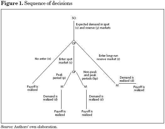
We will analyze the profit–maximizing behavior of a power plant as follows (see figure 1). There exists a sequence of decisions that any generation plant (GP) must take. First, after the decentralized ISO announces the expected demand for the next period,²² any generation plant must choose one of three possibilities: a) supply for the short–run spot market, b) offer capacity for the long–run reserve market, or c) stay out of the market. We restrict plants to choose only one of these alternatives. First, the generator might supply energy in the short–run market (or pool), or capacity in a long–run market for capacity reserves, or not supply at all. Second, if the generator decides to supply for the spot market, it must choose to sell energy only for the peak period (only for the peak hours, these plants are called "peaking plants"), or for both, peak and non–peak (offering energy all the time).²³ Once all gps have made their decisions, the market²⁴ plays and decides the actual demand for the three markets. After this, all GPS get their payoffs by computing their expected profits.

This is the more general context for analyzing the power plant's behavior in the spot and long–run reserve markets. A particular case would be the perfect competition model, where power plants entering the spot market are ordered by the decentralized ISO according to their bids. After that, they are dispatched until demand is satisfied. If we think of a vertically integrated system, then the perfect competition model is more accurate. However, if we think of a new market architecture, where plants will be free to choose, the model analyzed in this paper is better. It would allow getting the right implications; for example, the strategic behavior of plants trying to drive prices up in order to get higher profits.

The conditions that characterize the optimal behavior of generators under these scenarios should hopefully provide the decentralized ISO with key clues to evaluate the impacts of different pricing rules, that seek to enhance supply of energy and capacity reserves.

In order to analyze this mechanism, and following the sequence of decisions shown in figure 1, we use the tool of sequential games.

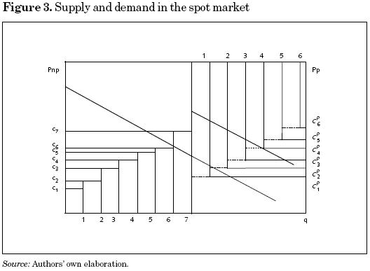
Definition 1: A sequential game is given by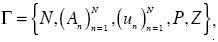

where:

(i) N is the set of players

(ii) A_n is the set of actions available for player n = 1,2,..., N

(iii) u_n is the payoff function for player n = 1,2,..., N

(iv) P is the player function

(v) Z is the set of histories in Γ

Therefore, in this mechanism we have the following elements. The set of N players is where so is the decentralized independent system operator, M is the market (its only role is to set the actual demand), and there are N — 2 power plants, denoted by GP_n. We assume plants are risk neutral.

The decentralized ISO's set of actions is A_so = [0, ∞) × [0, ∞). So, any pair d^e = (x, y) [0, ∞) × [0, ∞) denotes the expected demands in the spot and in the long–run reserve markets, respectively. The market's set of actions is A_m = [0, ∞), denoting the actual demand in any of these markets. The GP_n's set of actions is A_gp = {n, s, r, p, bp}for n = 1,2,..., N—2.

The set of histories is Z = {, d^e,d^en, d^es, d^er, d^erd, d^esp, d^esbp, d^espd, d^esbpd}.²⁵ For example, d^espd means that the decentralized ISO expects a demand d^e = (x, y), the GP decides to enter the sport market and supply energy for the peak period, and the market chooses an actual demand of d. The terminal histories are T = {d^en, d^erd, d^espd, d^esbpd}.²⁶ The non–terminal histories are NT = {, d^e, d^es, d^er, d^esp, d^esbp}.

The player function, defined as P : NTN, assigns one (o more) player (s) to any non–terminal history. Thus, P () = SO, P(d^e) = , P (d^e s) (in this case, the only power plants which are called to play are the ones that decided to enter the spot market), P (d^er) = M, P (d^esp) = M, and P (d^esbp) = M.

Finally, the payoff function for any power plant is given by its producer surplus, which will be defined below. In this context, actual demand and the bids made by all power plants participating in any particular market will determine the final prices.

Therefore, we will be looking for the equilibrium in this game, in particular, for a Perfect Subgame Nash Equilibrium,²⁷ which is stated as follows.

Definition 2. A strategy profile is a Subgame Perfect Nash Equilibrium if it is a Nash Equilibrium in each subgame.

Following definitions 1 and 2, we are looking for a configuration of plants in which no plant has incentives to move from one market to another. Based on this model, we will analyze if this mechanism has the right structure to give incentives to satisfy the actual demand in the spot market, and to expand the generation capacity in the long–run reserve market. Moreover, we can compare with the outcomes provided by the perfect competition model, where the strategic behavior is not possible.

II.1.1. Incentives for Expansion of Capacity

In this section, we will analyze the generation plant's strategic behavior in the short–run spot market. The only choice for them is to choose to generate electricity for the non–peak period or for both, the non–peak and peak periods, once they decided to enter the spot market. After finding the producer surplus they get in this market, we will allow plants to decide whether to generate for this market, or to offer capacity for the long–run reserve market, or to stay out of the generation market, by comparing the payoff they would get from these decisions. In this context, all generators will make their decisions depending on the expected profits they would get in each market.

II.1.1.1. The Spot Market

The spot market works as follows. Each generator decides voluntarily whether or not to participate in this market. Once it decides to participate, it chooses to supply for the peak, or for the non–peak and peak periods. The decentralized ISO coordinates the market with operations in real–time and forecasting for a time period in advance from an engineering technical scope, as well as from an economic perspective. Based on the expected demand for the non–peak period, each participating generator makes a merit order bid based on its capacity and costs. Then, in the real–time market, the decentralized ISO ranks the bids and offers economic dispatch service, based on marginal–cost power pricing. That is, generators are dispatched, according to their price bids, from the lowest to the highest one until demand is satisfied. After that, the market price in the non–peak period is the price bid of the last dispatched generator (called the marginal plant). For the peak period, the decentralized ISO and the participating generators (the earlier ones plus the peaking plants) follow the same rules.²⁸

Let us consider the following set up. There are N—2 generators. Each generator n = 1,2,..., N — 2 has a capacity of Q_n and a cost of C_n (Q_n).²⁹ Each generator makes a merit order bid based on Q_n and C_n. Suppose that each generator makes a bid of c_n for each unit of capacity that it is willing to supply. That is, generator n offers q_n units of capacity at a cost of c_n for each unit. Without loss of generality we suppose that c₁ < c₂ < ... < c_N—2. So, we have ordered plants according to their bids, and name them accordingly. The generation capacities for these plants are Q₁, Q₂,..., Q_N—2 and they could offer q₁, q₂,..., q_N—2 to the spot market. It is allowed to set q_n ≤ Q_n, so that power plants are not offering their total capacity. By doing this they could have a positive impact on prices, since following this strategy by the more efficient plants implies that more costly plants must be dispatched.

We now make the following assumptions. If the generator decides to participate in the spot market, it offers all capacity in the peak period, or in non–peak and peak ones; that is, q_n = Q_n. Let P=P(q) be the inverse demand function, which includes the peak load. We assume that this function is linear in both the peak and non–peak periods. This inverse demand function has the shape shown in figure 2. In this figure, we have ranked all generators according to their bids. The quantity supplied in the market is the sum of all quantities supplied by each of these plants. That is, the supply curve is the upward sloping step curve shown in this same figure. Then, price and quantity are defined according to the rules described above. For example, in this case the price in the non–peak period will be p^np = c_N—5, and the quantity supplied will be q^np = q₁ + q₂ + ... + q_N—6 + q_N—5. The additional quantity supplied for the peak period is q^p = q_N—4 + q_N—3, and the price would be p^p = c_N—3 > c_N—5= p^np.

From now on, we simplify this model furthermore. We assume that each plant has only one unit of capacity. This makes computation easier without loss of generality. In this context, we compute the market price for generation, the quantity supplied by generators, the producer surplus and the consumer surplus. Based on this information, each firm will decide to supply for the peak period or for both, non–peak and peak.

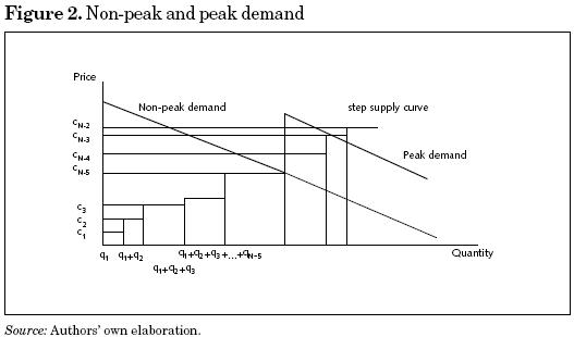
Thus, we have that q₁ = q₂ = ... = q_N—2 = 1. From the total number of generators, there are N_bp of them supplying in both non–peak and peak periods, N_p plants supplying only for the peak period, N_r supplying capacity for the long run reserve market, and N_o staying out of the market. This configuration of plants satisfies N_np+N_p +N_r +N_o=N—2. This situation is depicted in figure 3. In this figure, we do not show the offers made by the N_r participating in the long run reserve market. Therefore, given the demand function and the bids made by these generators, we get the following results.

There are seven plants choosing to supply energy for both periods. Their costs are c_n for n = 1,2,–,7. Given the actual demand, only six plants are dispatched. On the other hand, there are six plants offering capacity only for the peak period. Their costs are for for n = l,2,...,6. Considering the additional demand for the peak period, four more units are dispatched. Note that the seventh plant is out of the market, since its cost is higher than the costs of the first four plants in the peak period, even though it is making an offer for both periods.

For the non–peak period (this includes only plants supplying energy for peak and non–peak periods) we have the following results. The price, paid to these plants, set by the marginal plant (plant 6) is

and quantity is

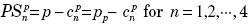
The producer surplus is

and total producer surplus is

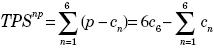
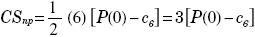
Finally, consumer surplus is

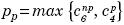
For the peak period we have the following (this includes all plants supplying energy for the spot market). In this case, the marginal plant (plant 4) has a bid of . This is the case shown in figure 3. The price prevailing in the peak period will be the one set by the marginal plant; that is, the maximum between c₆ and . Therefore, the price in the peak period will be

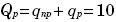
Quantity has increased by units. So, total quantity is

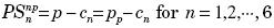
Additional producer surplus, obtained by the peaking plants, is

the additional surplus obtained by plants that supply energy all the time is

and additional consumer surplus:

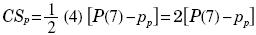
Therefore, total producer surplus is

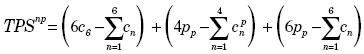
and total consumer surplus is

So, we have that p_np ≤ p_p, which is the result we should expect.

Let us analyze the behavior of plant 1 in this market. Its decision of offering only for the peak, or for the non–peak and peak periods, depends on the marginal plant in each period. Given that c₆ < , we have p_np < p_p. Then, this plant gets a higher producer surplus by offering energy in the peak period, since PS₁^np = p_np – c₁ < p_p – c₁ = PS₁^p. For the same arguments, all plants offering for both periods have incentives to move to the peak period only.³⁰ This strategic behavior would induce an increase in the price of the non–peak period. On the other hand, it could also be that p_np = p_p (which would seem a strange case for electricity markets. However, consider the following scenario. Many plants with very low bids decide to offer energy only for the peak period. In this case, the price in the peak period will be the same as that of the marginal plant setting the price in the non–peak period). In this case, all plants are indifferent between the two decisions. Thus, all plants will decide depending on the cost of the marginal plant being dispatched in each period. Therefore, the actual prices for the non–peak and the peak periods depend on the configuration of plants choosing to serve each period.

Let and be the bids of the marginal plants dispatched in the non–peak and peak periods, respectively. Then, we have that ≥ 0 for k= n p, p. That is, the higher (lower) the bids of these plants, the higher (lower) the producer surplus of all plants in that period. Therefore, the incentives to move from one period to the other will depend on the configuration of each set of generators. No plant will move if = .

Finally, by the arguments discussed above, an equilibrium in this market is a configuration of plants {N^*_np, N^*_p} such that = .³¹ This gives a Nash Equilibrium³² in this market, since no plant has incentives to move from one period to the other. So, total expected demand is satisfied in non–peak and peak periods. Moreover, we get that = , which is the stable equilibrium, since the model gives the right incentives to get this result whenever prices are different. It is important to note that this result could not prevail if there were some frictions, such as impossibility to move among markets. One important case where we find different prices, more generally <, is the perfect competition market, where all plants are ordered according to their bids. Therefore, in vertically integrated markets we expect that prices will be higher in the peak period. However, there are other possibilities as we find in this model.

Now we proceed to analyze the long–run reserve market. In this case, we compute the expected profits of a generator that decides to offer capacity in this market. We then compare these profits with profits it would get in the short run spot market. Based on this, the generator will decide the strategy that maximizes its profits.

II.1.1.2. The long–run reserve market

In this section we model the behavior of the generation plants that choose to supply capacity for the reserve market in the long run. This is an uncertain market, since the size of the additional demand at that particular point in time is unknown. All plants deciding to participate in this market have a probability of being dispatched. The bigger the additional capacity demanded in this market at that time, the higher the probability of being dispatched. Clearly, given the merit order mechanism, the generator with the lowest bid will be dispatched for sure. For the other plants, it will depend on the combination between the size of the actual increase in demand at that moment in time, and the cost configuration of all power plants choosing that market.

In order to analyze this market, we construct a simple model that gives us some hints of what could happen. We assume that additional demand might be y = 1,2,3,..., Y units of electricity. There exists a probability distribution over this additional demand; the lower the quantity, the higher the probability. Let P be a probability distribution over Y given by . So, p_y is the probability of having an additional demand of y for y = 1,2,3,..., Y where p₁ > p₁ > ... > p_y, p_y> 0 for y = 1,2,3,..., Y and p_y=1.

Suppose that each plant, n, entering this market makes a bid. It will offer one unit of capacity at a cost of c_n. Once all plants willing to supply capacity for the long run reserve market make their offers, they are ranked according to their bids. Say we have N_r plants in the market. Then, the ordering will be < < ... < . Given this ordering, we compute the expected producer surplus for entering this market.

Plant 1 will get with probability p₁, – with probability p₂, – with probability p₃, and so on. That is, recalling that it is risk averse, it will get an expected producer surplus of = p_y ( – ). Thus, plant n will get an expected profit of = p_y – .

Therefore, we have the following results in this market. First, < 0; that is, the lower the costs of plant n, the higher the expected profits. Then, the less costly plants are the ones that are more likely to enter this market. Second, if we have a probability distribution given by _y where ₁ > ₂ > ... > _N, _y > 0 for all y = 1,2,3,...,Y and _y = 1 that is stochastically dominated by the probability distribution P, then the expected profits for all generators will be higher under P than under . Therefore, the higher the expected demand, the higher the expected profits in the long–run reserve market. In this case, more generators will be willing to supply capacity for this market. Third, > 0. That is, the bigger the difference between the n's bid and the bids of the other firms (which are more costly), the higher the expected profits of generator n. Therefore, the less costly generators, with respect to all generators in the market, are the ones that are more likely to enter this market.

Finally, we compare these expected profits with the profits in the short–run spot market. Think of generator 1, the less costly one, for the case depicted in figure 3, above.

In the non–peak period, it would get c₆ – c₁. In the peak period, it would get – c₁. In the long run reserve market, it would get = p_y – c₁. Given that c₆ < , it prefers the peak period than the non–peak period. However, if p_y >, this generator will prefer to supply capacity for the long–run reserve market. That is, if the average expected cost in the long run reserve market is bigger than the price bid of the marginal plant in the peak period, then generator 1 would get higher profits in the long–run reserve market. So, plant 1 will choose to supply capacity for the long–run reserve market. Therefore, we have the following general result.

Proposition 1: The Subgame Perfect Nash Equilibrium in this game is a configuration of plants {N^*_o, N^*_s, N^*_r}, such that N^*_o+ N^*_s + N^*_r = N–2 and N^*_np + N^*_p = N^*_s, where no plant has incentives to move. That is, where = = p_y .

Finally, based on these profits, we see that there are incentives for building more capacity for the reserve market for two reasons. First, new potential generators would use better technologies, which imply lower costs and higher expected profits for them. Second, given that demand is growing over time, the more costly plants will likely be dispatched even though more capacity is installed. The only case when these more costly plants are displaced from the market is when the growth rate of demand is lower than the growth rate of new capacity. In this case, there would be gains in consumer surplus, since the new generation is entering at lower cost and, therefore, there would be lower generation prices.

Moreover, in the long run this new capacity would enter the non–peak period, the peak and the long run reserve market, depending on the configuration of plants that are generating electricity at that moment in time. These new plants will get producer surplus that is strictly positive. It would be a matter of choice whether they enter the spot market or the long run reserve. This decision would depend on the market prices that are expected to prevail in each one. However, it is important to note that generation prices could not decrease over time if the expansion in capacity grows at the same or lower rate than demand. Finally, there is room for strategic behavior since plants always have incentives to drive prices up by moving from one market to another (it is easy to find markets with such characteristics).

 

III. Simulation

In this section we make a simulation to compute the generation cost in Mexico for 2004. We want to find the minimum generation cost, according to the merit model discussed above, and compare it with the actual cost for the Mexican electricity sector. All data used in this exercise come from CFE. The year used for comparison is 2004 only for the interconnected system.³³ Total installed capacity (in MW) is given for each technology. The load factor (the efficiency of the power plant) is the weighted average for each technology depending on the capacity of each plant. Load factors for 2003 are used for the computation in 2004 (we think there is no problem, since there is almost no change from year to year). One important caveat applies for hydroelectricity, since the load factor depends on the previous raining season and could imply some bias in the computation of the weighted average.

On the other hand, demand is needed to compute the amount of power required for the peak and non–peak periods. It is classified in three groups: a) base demand, which is required 24 hours a day; b) intermediate demand, which is required during some hours almost all days a year; finally, c) peak demand, which is required for some hours some days a year. For 2004 we have the following estimation. Total demand is 212 480.47 GWh. Base demand is 187 837.06 GWh, intermediate demand is 12 179.11 GWh and peak demand is 12 464.3 GWh (this is the additional demand that we modeled in our game and appears in figure 3 as 4 extra units). We classify the first two as non–peak and the last one as peak demand for our simulation. Therefore, the non–peak demand is 200 016.17 GWh and the peak demand is 12 464.3 GWh. Finally, since 10 per cent of total demand is satisfied by self supply, cogeneration, etc., we used only 90 per cent of the total demand reported for 2004 for our estimation.

Finally, data about costs, load factors and capacity for each technology is presented in table 1. Also, following the merit order model, this table shows the dispatch order for each one.

We use monthly data for 2004 as our simulation exercise, by using a seasonality factor computed from the total generation in that month. Table 2 shows the results for this simulation.

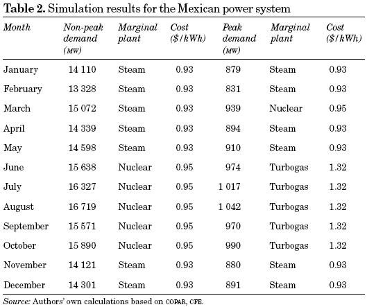
Following the merit order dispatch, the cost of generation in the peak period is higher than the cost for the non–peak period. This is the case because the Mexican power system is a vertically integrated market, where all decisions are made by the so. If plants were allowed to move from one market to another, we might get the result predicted by our model. Once the generation plants observe these prices, they will have incentives to move from the non peak to the peak period. In this way, the price will equalize after some lower cost plants go to the peak period.

On the one hand, there is some monthly seasonality in the consumption of electricity. The highest consumption is during July and August. The lowest consumption months are from January to May. In January, February, April and May, the marginal plants in both periods are the steam ones. Therefore, the generation cost is the same for peak and non peak periods. In March, the marginal one is the nuclear. For the other months, there are differences in the marginal plants during the peak or non peak periods. In these cases the cost is higher for the peak one. In a fully open generation market, we could expect some movement of plants from the non peak to the peak period, as stated in proposition 1. Therefore, the results predicted by proposition 1 hold, depending on the actual sizes of demand in non–peak and peak periods.

On the other hand, during July and August the reserve margin is only 1 per cent, while for June and September the reserve margin is 5 per cent. In these four months we do not have a reliable system, because the reserve margin is below international standards, given by 6 to 9 per cent. So, the Mexican power system was lucky not to have any disturbance in its system.

Finally, we compare our simulation with data reported by CFE about total generation in 2004. This allows us to reach some conclusion about the performance of the system. That is, to know if CFE is following the merit order model for dispatch. Table 3 shows actual total generation and simulated generation by technology.

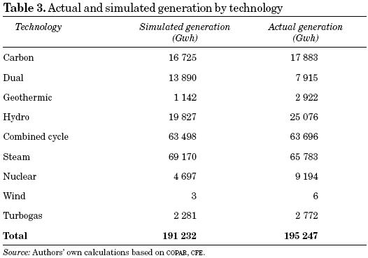
There are some differences between our simulation and the actual generation. The most important ones are the hydro, dual and nuclear technologies. For the hydroelectricity, the possible explanation is that the load factor we used in our simulation is smaller than the actual one. This is a possibility, if we think that 2003 was a wet year. In that situation, the load factor for these plants can be bigger. However, this could be a special year. It is no guarantee that this will happen all years. The differences for the dual technologies could reflect congestion problems because, in general, these are located in the most congested zones. Therefore, CFE could decide not to dispatch some of them and replace by more costly ones. On the other hand, these plants were replaced by hydro ones, due to the argument above. Finally, nuclear generation is smaller in our simulation because the starting cost of this technology is so high, that the best strategy is to dispatch this plant all the time. Moreover, since its capacity is needed during six months, the best strategy is to put it in all the time. Finally, there exists a small difference in total generation, which is not so relevant.

 

IV. Conclusions

Ideally, the energy and the reserve markets should not be separated, and the so could run day–ahead markets and spot markets that take care of imbalances and reach equilibrium of all electricity markets in an integrated way. Market players would then meet their long run expectations on demand–supply balance in well–developed forward markets. That is, energy and reserve pricing would take care of supply adequacy. However, in practice electricity markets are sometimes implemented together with transitory resource–adequacy policies. Capacity payments and requirements present several inconveniences both in theory and practice. The most advanced developments in the literature point to combine them with some type of hedging instruments, such as call options, so that regulatory intervention is focused on promoting liquid markets for energy risk management.

Following this discussion in the literature, we proposed a simple model to explain the strategies of the generation plants in the spot market, together with the long run reserve market, to satisfy the expected demand. We found the expected costs of generation in the spot market, for the non peak and the peak periods, and in the long–run reserve market. We then compared our simulated dispatch with the actual dispatch for the Mexican electricity system for 2004. There are some disparities that can arise because of differences in the load factor, congestion costs or entry costs, which are omitted from our simulation. However, the total generation is very similar. But the fact that total generation is similar to that in practice does not really prove how realistic the modeled prices and dispatch order are. What is shown is that the model is a good approximation that needs to be strengthened furthermore, in order to incorporate some of the shortcomings discussed above. Moreover, we should compare actual and simulated total costs to get more robust results. So, if data about generation tariffs were available, it could be possible to compare them with simulated tariffs.

Mexico does not currently have an open market. Only in recent years CFE argues that a mock (or shadow) market has been implemented inside the vertical integrated state monopoly. This virtual market seeks to emulate a competitive market. It uses an optimization model where the least–cost dispatch is based on actual generation costs (merit order rule) in one–day–ahead and real–time markets. The one–day–ahead market establishes production, consumption and price schedules for each of the hours of the following day. The differences between forecasted and actual schedules are cleared at real–time prices. Bids are actually submitted to the system operator (CENACE) by the different "programmable" thermal CFE's generation plants, which are administratively separated so that they function as different power producers.³⁴

In this virtual market, payments to generators include a "capacity" payment intended to foster the development of generation capacity reserves. It then seems that the combination of this virtual market (with still some elements of central control and subsidy scheme of the state–owned holding company), together with capacity payments, has eventually resulted in capacity generation expansion similar to what would be attained in an open electricity market, as the one modeled in our study. But this by no means proves that the Mexican electricity industry will not need in the future some of the additional capacity expanding mechanisms discussed in this paper.

Our model, that simulates a "market" solution to assure resource adequacy, has also some simplifying assumptions that should be relaxed in a more general setting. First, plants have only one unit of capacity. This assumption eliminates problems about capacity payments and strategic behavior trying to push price up in one of the three submarkets. Second, plants are risk neutral and there is not discount. This assumption assures enough capacity for the long–run reserve market. Third, we ignore the rest of the electricity system, avoiding possible congestion in the transmission lines, among others.

Finally, this is a static setting. Plants have no chance to move from one submarket to other over time, and costs for different technologies might vary over time. In addition, in a dynamic setting the long–run peak–period price could be expected to intertemporally attract investments ("calling effect"). Therefore, we cannot conclude that any electricity system does not need an additional mechanism to assure resource adequacy, or that the "market" is the "right" mechanism.

 

References

Borenstein, S. (2002), "The Trouble With Electricity Markets: Understanding California's Restructuring Disaster", Journal of Economic Perspectives, 16, pp. 191–211.         [ Links ]

Bouttes, J. P. (2004), Roundtable "Market Design and Competition in Electricity", presented at IDEI–CEPR conference "Competition and Coordination in the Electricity Industry", January, pp. 16, 17.         [ Links ]

Carreón–Rodríguez, V. G., Jiménez San Vicente, A. and J. Rosellón (2007), "The Mexican Electricity Sector: Economic, Legal and Political Issues", in David G. Victor and Thomas C. Heller (eds.),The Political Economy of Power Sector Reform: The Experiences of Five Major Developing Countries, Cambridge University Press.         [ Links ]

Chandley, J. D. and W. W. Hogan (2002), "Initial Comments of John, Chandley and William Hogan on the Standard Market Design NOPR", November 11, available at: http://ksghome.harvard.edu/~.whogan.cbg.Ksg/.         [ Links ]

Chao, H. P. and R. Wilson (2002), "Multi–Dimensional Procurement Auctions for Power Reserves: Robust Incentive–Compatible Scoring and Settlement Rules", Journal of Regulatory Economics, 22(2), pp. 161–183.         [ Links ]

Comisión Federal de Electricidad (2001), Costos y parámetros de referencia para la formulación de proyectos de inversión en el sector eléctrico.         [ Links ]

–––––––––– (2005), Costos y parámetros de referencia para la formulación de proyectos de inversión en el sector eléctrico.         [ Links ]

Creti, A. and N. Fabra (2004), "Capacity Markets for Electricity", Working Paper, 124, UCEI, CSEM.         [ Links ]

Davis, T. (2004), "New England Officials, Utilities Yowl Over Installed Capacity Plan", The Energy Daily, March 24.         [ Links ]

De Vries, L. J. (2004), Securing the Public Interest in Electricity Generation Markets: The Myths of the Invisible Hand and the Copper Plate, Ph. D. Dissertation, The Netherlands, Delft University of Technology.         [ Links ]

De Vries, L. and K. Neuhoff (2003), "Insufficient Investment in Generating Capacity in Energy–Only Electricity Markets", paper presented at 2nd Workshop on Applied Infrastructure Research (Regulation and Investment in Infrastructure Provision–Theory and Policy), TU Berlin WIP, DIW Berlin, October 11.         [ Links ]

Doorman, G. (2000), Peaking Capacity in Restructured Power Systems, Thesis (Ph.D.), Norwegian University of Science and Technology, Faculty of Electrical Engineering and Telecommunications, Department of Electrical Power Engineering.         [ Links ]

Federal Energy Regulatory Commission (FERC) (2002), Notice of Proposed Rulemaking: Remedying Undue Discrimination through Open Access Transmission Service and Standard Market Design, Docket No. RM01–12–000, July 31.         [ Links ]

Green, R. (2004), "Did English Generators Play Cournot?", mimeo, University of Hull Business School.         [ Links ]

Gülen, G. (2002), "Capacity Payments", presentation, 22nd Annual IAEE/USAEE North American Conference, Vancouver, October 6–8.         [ Links ]

Harvard Electricity Policy Group (2003), "Rapporteur's Summaries of HEPG Thirty–First Plenary Session", May, pp. 21–22.         [ Links ]

Hobbs, B. F., J. Iñón and S. E. Stoft (2002), "Installed Capacity Requirements and Price Caps: Oil on the Water or Fuel on the Fire", The Electricity Journal, July, pp. 23–34.         [ Links ]

Hobbs, B.F., J. Iñón and Kahal, M. (2001), A Review of Issues Concerning Electric Power Capacity Markets, Project report submitted to the Maryland Power Plant Research Program, Maryland Department of Natural Resources, Baltimore, The Johns Hopkins University.         [ Links ]

Hunt, S. (2002), Making Competition Work in Electricity, New York, John Wiley & Sons.         [ Links ]

International Energy Agency (IEA) (2002), Security of Supply in Electricity Markets: Evidence and Policy Issues, OECD/IEA.         [ Links ]

Joskow, P. (2003), "The difficult transition to competitive electricity markets in the US", Working Paper, The Cambridge–MIT Institute Electricity Project, CMI 28,         [ Links ]

Joskow, P. and J. Tirole (2004), "Reliability and Competitive Electricity Markets", paper presented at IDEI–CEPR conference "Competition and Coordination in the Electricity Industry", January, pp. 16–17.         [ Links ]

Knops, H. (2002), "Electricity Supply: Secure under Competition Law?" proceedings, 22nd Annual IAEE/USAEE North American Conference, Vancouver, October 6–8.         [ Links ]

Madrigal, M. and F. De Rosenzweig (2003), "Present and Future Approaches to Ensure Supply Adequacy in the Mexican Electricity Industry", paper presented at the Power Engineering Society Meeting, IEEE, vol. 1, pp. 540–543, Toronto, July 13–17.         [ Links ]

Newbery, D. M. (1995), "Power Markets and Market Power", The Energy Journal, 16 (3), pp. 39–66.         [ Links ]

Oren, S. (2000), "Capacity Payments and Supply Adequacy in Competitive Electricity Markets", in Proceedings of the VII Symposium of Specialists in Electric Operational and Expansion Planning, Curitiba (Brazil), May 21–26.         [ Links ]

–––––––––– (2003), "Ensuring Generation Adequacy in Competitive Electricity Markets", Energy Policy and Economics Working Paper, UCEI, EPE 007.         [ Links ]

Oren, S. and R. Sioshansi (2003), "Joint Energy and Reserves Auction with Opportunity Cost Payment for Reserves", paper presented at IDEI–CEPR conference "Competition and Coordination in the Electricity Industry", January, pp. 16–17.         [ Links ]

Osborne, M. J. and A. Rubinstein (1994), A Course in Game Theory, The MIT Press.         [ Links ]

Patton, D. S. (2002), "Review of New York Electricity Markets", New York Independent System Operator, October 15, Summer.         [ Links ]

Pennsylvania, Maryland, and New Jersey ISO (PJM) Monitoring Market Unit (2003), "State of the Market Annual Report", available at: http://www.pjm.com.         [ Links ]

Singh, H. (2002), "Alternatives for Capacity Payments: Assuring Supply Adequacy in Electricity Markets", presentation, 22nd Annual IAEE/USAEE North American Conference, Vancouver, October 6–8.         [ Links ]

Stoft, S. (2002), Power System Economics: Designing Markets for Electricity, Wiley–IEEE Press.         [ Links ]

–––––––––– (2003), "The Demand for Operating Reserves: Key to Price Spikes and Investment", IEEE Transactions on Power Systems, 18(2), May, pp. 470–477.         [ Links ]

Vázquez, C., M. Rivier and I. Pérez Arriaga (2002), "A Market Approach to Long–Term Security of Supply", IEEE Transactions on Power Systems, 17, May, pp. 349–357.         [ Links ]

Wilson, R. (2002), "Architecture of Power Markets", Econometrica, 70, pp. 1299–1340.         [ Links ]

 

Notas

We are grateful to William Hogan and an anonymous referee for insightful comments. Rosellón acknowledges support from the Repsol–YPF–Harvard Kennedy School Fellows program, the Fundación México en Harvard, and the Comisión Reguladora de Energía.

¹ Reliability in electricity markets is understood as the sum of adequacy and security standards. Adequacy (security) is associated with the long run (short run). Security describes the capability of the system to deal with contingencies, and includes the so called ancillary services. Adequacy addresses the ability of the system to continuously meet the consumer energy requirements (Singh, 2002; Oren, 2003).

² De Vries and Neuhoff (2003) carry out an extensive analysis of the market and institutional failures in the electricity industry.

³ Stoft (2002) explains how a market with a perfectly inelastic demand function can still achieve the socially optimal volume of generating capacity.

⁴ Demand is not always only inelastic due to regulated tariffs. In many countries, consumer rates are not regulated. However, if meters are read only annually (or monthly), it is not possible to distinguish the time of electricity consumption, and consumers still do not have a short–term reaction to prices.

⁵ In Norway, there is direct State ownership of some peaking plants (Gülen, 2002).

⁶ For instance, in the United States gas cost allocation to charges has varied from an "Atlantic Seaboard" method, which assigned 50 per cent (later 100%) of fixed costs to the commodity charge, to the "Straight Fixed Variable" method, which allocates all fixed costs to the capacity charge.

⁷ See also Newbery (1995).

⁸ PJM initiated monthly and multi–monthly capacity markets in 1998, while daily capacity markets started in 1999. See Hobbs, Iñón and Kahal (2001) for an in depth analysis of ICAP issues in PJM.

⁹ Joskow and Tirole (2004) also propose a model which combines capacity requirements with capacity price caps, that might potentially restore investment incentives.

¹⁰ For instance, in the New York ISO a demand curve is constructed as an alternative to valuing an additional ICAP above the fixed capacity requirement (Harvard Electricity Policy Group, 2003).

¹¹ PJM solved its problem of capacity leaking to neighbouring systems, by requiring generating companies to commit for longer periods, if they wanted to sell ICAP credits.

¹² The average scarcity rents in New England of $10,000 MW–Year, are very low when compared to the fixed cost of a new reserve capacity facility, estimated in between $60,000–$80,000 MW–year (Joskow, 2003).

¹³ Creti and Fabra (2004) deduce, from their theoretical model, the possibility that capacity markets clear at zero prices, if there is no spread between national and foreign prices.

¹⁴ Doorman (2000) suggests an alternative capacity mechanism, based on capacity subscriptions.

¹⁵ Alternatively, LSEs could be the buyers of options through bilateral contracts with generators.

¹⁶ Option premiums work as substitute efficient signals, compared to price signals generated by capacity requirements (Singh, 2002).

¹⁷ A specific call–option mechanism for the electricity market in Colombia is proposed in Vázquez, Rivier and Pérez Arriaga (2002). The regulator requires the system operator to buy a prescribed volume of reliability contracts, which allow consumers to get a market compatible price cap in exchange for fixed capacity remuneration to generators. Reliability contracts then consist of a combination of a financial call option with a high strike price, and an explicit penalty for generators in case of non–delivery. The regulator carries out a yearly auction of option contracts, and sets the strike price (at least 25 per cent above the variable cost of the most expensive generator) and the volume of capacity to be auctioned. Generators de CIDE how to divide their total capacity and price into different blocks, so that capacity assigned to each generator is a market result rather than an administrative outcome. This proposal is very sensitive to market power. Therefore, implementation requires that the maximum amount a generator can bid is limited to its nominal capacity. Likewise, portfolio bidding is not allowed, and the winning bids cannot transfer their obligations of physical delivery to other generators.

¹⁸ The ISO has a natural monopoly over its functions. Several design issues arise regarding the ISO's organization and institutional characteristics, such as governance, incentives, regulation, and economic objective functions. Regarding congestion of transmission lines, the objective function of an ISO should consider the minimization of difference in nodal prices, and the maximization of total energy traded in the electricity system.

¹⁹ Hybrid designs allowing for different degrees of centralization are also possible: central control of transmission and reserves by an ISO, together with forward markets for energy.

²⁰ We also assume, for simplicity, that the decentralized ISO takes care of financial transactions in addition to the physical operations of the system. That is, the ISO also carries out the "PX" functions. In practice, these functions can of course be separated.

²¹ In practice, generation plants with market power might carry out bid strategies, in order to increase the spot price. According to Stoft (2002, pp. 320–322), some of these strategies include quantity distortions (output is decreased below its competitive level), price distortion (price is increased above its competitive level) and quantity withholding (producing less than would be profitable).

²² We abstract from any specific time span, since we want to stress the behavior of power plants when deciding about any of the submarkets.

²³ In this model, we allow plants to decide between "peak", and "non–peak and peak". Although this is an analytical assumption, it helps to approximate a model to the peaking plants and base–load plants practice behavior of electricity markets.

²⁴ We introduce "the market" as a player to illustrate that the environment plays an important role in determining actual demands (in the spot market and in the long run reserve market). Actual demands could differ from the expected ones forecasted by the decentralized ISO.

²⁵ The variable denotes the beginning of the game. That is, there is no history behind; no player has been called to play.

²⁶ We define a terminal history as a history where no player is called to play. After any of these histories, payoffs are realized. By the same token, we define a non–terminal history as a history where there is time for one of the players to play.

²⁷ For a more complete development of a sequential game, as well as Nash and Perfect Subgame Nash Equilibrium, see Osborne and Rubinstein (1994).

²⁸ It is important to note that this mechanism minimizes generation costs in both periods.

²⁹ This cost includes the capacity fee and the energy fee.

³⁰ We say that plants could move from the "non–peak and peak" periods to the "peak" period, in the sense that some plants might wish to become peaking plants only. However, this would be rare for the case of base–load plants, such as nuclear, geothermal or coal plants. This statement would therefore make more practical sense for plants using natural gas. Therefore, we should expect that combined cycle plants would be the peaking plants.

³¹ The case of equal prices in peak and non–peak periods is an extreme analytical case of no base–load technology (such as nuclear plants), and only peaking power plants. This by no means reflects the practice of electricity markets. However, this result is very important because it gives the right incentives to supply energy in the spot and long-run reserve markets, and sheds light on the strategic behavior of plants to drive prices up.

³² See Osborne and Rubinstein (1994) for the concept of Nash equilibrium and the logic behind it.

³³ Baja California is not connected to the rest of the country. For this reason, we eliminate in the simulation both its supply and demand. We also eliminate other small subsystems.

³⁴ "Non-programmable" generators are small producers that only supply power according to a previously set energy delivery schedule.