Notas

 

Halving Poverty in Mexico

 

¿Es factible disminuir a la mitad la pobreza en México?

 

Juan Carlos Chávez–Martín del Campo¹ and Manuel Gómez²

 

¹ Profesor–investigador de la Escuela de Economía, Universidad de Guanajuato, UCEA–Campus Marfil, Fracc. I, El Establo, 36250, Guanajuato, Gto., México. juancarlos.chavez@ugto.org.

² Profesor–investigador de la Escuela de Economía, Universidad de Guanajuato, UCEA–Campus Marfil, Fracc. I, El Establo, 36250, Guanajuato, Gto., México. manuel.gomez@ugto.org.

 

Fecha de recepción: 3 de octubre de 2007.
Fecha de aceptación: 28 de mayo de 2008.

 

Abstract

We estimate the required time and the minimum necessary growth rate to halve poverty incidence and poverty intensity in Mexico's rural and urban areas for a series of counterfactual distribution and growth scenarios. Results show that, given the current income distribution, per capita incomes in the rural area would have to grow faster –in some cases eight times faster– than they have done historically to shrink poverty by half by 2015. In contrast, income in the urban sector would have to grow around 1 per cent per year to reach the same goal, which seems a more reasonable outcome given its behavior in past years.

Keywords: economic growth, millennium development goals, poverty goals, poverty measurement, Mexico.

 

Resumen

Estimamos el tiempo requerido y la tasa de crecimiento mínima necesaria para disminuir a la mitad la incidencia y la intensidad de la pobreza en las áreas rurales y urbanas de México, para diversos escenarios de distribución del ingreso y tasas de crecimiento. Los resultados muestran que, dada la distribución actual del ingreso, el ingreso per cápita en las áreas rurales tendría que crecer más rápido –en algunos casos ocho veces más rápido– que lo que ha crecido históricamente para disminuir la pobreza a la mitad en el año 2015. En contraste, el ingreso en las áreas urbanas solamente tendría que crecer alrededor de 1 por ciento anual, lo que parece un resultado más factible dado el comportamiento observado en años anteriores.

Palabras clave: crecimiento económico, objetivos de desarrollo del milenio, objetivos de pobreza, medidas de pobreza, México.

JEL classification: D31, I32, O40.

 

Introduction

Poverty goals are key indicators to evaluate the advancement of development. For instance, in September 2000 the world leaders of the United Nations adopted a document known as the Millennium Declaration, which explicitly set an ambitious agenda for international development. It includes a series of goals known as the millennium development goals (MDG).¹ The first of them establishes that countries should reduce by half: 1) the proportion of people living below $1 a day, and 2) the proportion of people who suffer from hunger, by 2015, taking the level observed in 1990 as a reference point. Since then, several approaches have been suggested and implemented to study the feasibility of that goal, for example Besley and Burgess (2003), Deaton (2003), and Chen and Ravallion (2004).

This paper develops and applies a simple methodology to estimate two parameters of interest for the analysis of poverty goals: the required time and the minimum necessary growth rate to meet a poverty goal under several growth and distribution scenarios. The methodology has several advantages. First, it can be applied to practically all poverty measures used in applied work. Second, the parameters of interest can be estimated on a case by case basis instead of estimating a cross–country regression. As noticed by Bourguignon (2002), this approach is more appropriate since both the development and the inequality levels of a country do affect the growth elasticity of poverty reduction. Third, the parameters can be estimated from aggregate data. These parameters are estimated for rural and urban Mexico in the case in which poverty goals imply halving both incidence and intensity of poverty in the middle–run.² To this end, we use not only the one dollar a day poverty line, but also the official food poverty lines and the two dollar a day poverty line, to take into account country–specifics.

The article is organized as follows: section I describes the methodology. Section II illustrates it using data from Mexico. Finally, section III summarizes the main results and conclusions.

 

I. Methodology

Let F_t(y) be the cumulative income distribution, and y_t (p) the p quantile of that distribution at time t. We focus on poverty measures that can be fully characterized in a general form as follows:

where μ_t is the mean income, z the poverty line and L_t the Lorenz curve.

As a special case for this class of measures, we have the family of addi–tively separable poverty measures, which can be written as:

where π(.) is the poverty evaluation function and H_t the proportion of people whose incomes are below the poverty line, z.³ For instance, the Foster–Greer–Thorbecke (1984) family of poverty measures is:

Let P* be a poverty goal. The needed mean income, μ*, to meet this poverty goal for a given income distribution, L, and an exogenous poverty line, z, is defined as:

Therefore, the time taken to meet the poverty goal, P*, given μ, L, z, and an annual per capita growth rate, , can be written as follows:

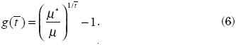
Analogously, the minimum necessary growth rate of per capita income, g (), to meet the poverty goal, P*, in years, holding both the income distribution and the poverty line constant is:

Incorporating Inequality into the Analysis

Although most of the poverty changes are explained by growth in average incomes, Kraay (2006) shows that changes in income inequality may play an important role in meeting poverty goals in the medium to long–run, particularly in very unequal societies. Nevertheless, incorporating changes in inequality into the analysis creates a further dilemma, given that the income distribution can change in an infinite number of ways.

To handle this problem, we use the lognormal distribution to approximate the distribution of income. This is a standard parameterization in applied work, because it fits the data very well and is tractable (López and Servén, 2006).

Exploiting the one to one mapping that arises under lognormality between the Lorenz curve and the Gini coefficient, G, and using the fact that L_t(p) = Φ (Φ^–1 (p)–σ_t) –see Aitchison and Brown (1966)–, it can be shown from (2) that:

where

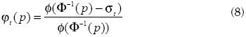
and

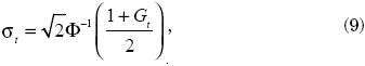
where Φ(.) and (.) are, respectively, the cumulative distribution function and the probability density function for the standard normal. Particularly, the Headcount ratio can be reformulated as:

It can be easily shown that < 0. Therefore, for a given G we have a unique average income, μ* (G), that solves.

From this equation we can estimate the parameters of interest, t() and g(), for counterfactual income distributions.

 

II. Meeting the Millennium Development Goals and Beyond in Mexico

We illustrate the methodology developed in this paper through the empirical analysis of the first MDG for Mexico: to eradicate extreme poverty and hunger. This goal breaks down into two targets: 1) to halve the proportion of population with an income below one dollar a day, and 2) to halve the proportion of population suffering hunger. These two targets should be accomplished no later than 2015, and their reference year is 1990. Besides halving the proportion of population whose income is below $1 ppp (Purchasing Power Parity) dollar a day, the Mexican government has explicitly compromised to halve the proportion of people in rural and urban areas living below the official poverty lines (Presidencia, 2005).

For the empirical application, we have chosen the Elliptical Lorenz curve ofVillaseñor and Arnold (1989):

where e = –(a+b+d+1), α = b² –4a and β = 2be–4d.⁴ This parametric representation performs very well relative to other functional forms, and it is analytically tractable. It has been used by Datt and Ravallion (1992) and Ravallion and Huppi (1989) to study growth and redistribution components in poverty changes. Estimators for the vectors of parameters (a, b, d) can be obtained by estimating the lineal model

where v is a random error process.⁵

We use the Mexican household survey ENIGH for the years 1992 and 2005 to obtain the necessary information on household incomes and demographic data for our estimates. The ENIGH is composed of two subsamples, representative, respectively, of rural and urban areas. We calculate individual incomes using the methodology of the National Council for the Evaluation of Social Policy (CONEVAL).

Three different poverty lines are used in this empirical application: 1 and 2 ppp dollars a day,⁶ and the official Mexican poverty lines proposed by CONEVAL, that reflect nourishment necessities in communities with less than 2,500 inhabitants (rural) and more than 2,500 (urban): 584.34 and 790.74 constant pesos of August 2005,⁷ respectively. We use 1992 as a reference year since the ENIGH was not carried out in 1990. In this year, the proportion of people living with less than one dollar a day was 13.4 and 0.8 per cent; the proportion of people not meeting their daily nourishment necessities was 35.6 and 13.4 per cent, in rural and urban areas respectively.

The period 2000–2005 was not characterized by high growth rates. Rural and urban average incomes registered annual growth rates of around 0.3 and 1.1 per cent, respectively. In 2005, average income in the rural sector was 1,221.9 pesos, while that in the urban sector was 3,002.7 pesos. These numbers will be useful to obtain the required growth rates to halve poverty in Mexico.

Table 1 provides estimates for halving the proportion of people living under the one dollar a day poverty line (poverty incidence) for both rural and urban areas. Assuming a constant income distribution through time, average income in the rural and urban sectors should rise to at least 1,563.6 and 1,704.4 pesos to halve poverty in 2015; this implies an annual growth rate of around 2.5 and –5.5 per cent respectively. For the rural area, it represents to grow over eight times faster than the average rate observed during the period 2000–2005. For the urban area, we estimate a negative growth rate because the goal has been met already –the required average income is only 1,704.4 pesos. We estimate a negative lower bound to meet the goal by 2015: –5.5 per cent, that is to say, ceteris paribus, the urban sector could register negative growth rates all over the period and still be able to meet the MDG. These findings are consistent with the fact that in Mexico, a relatively rich country among the developing economies, extreme poverty is mostly a rural phenomenon.

We also estimate the required number of years to meet the first MDG for several growth scenarios. If annual growth rates were in the order of 1, 3, 5 and 7 per cent, it would take 24.8, 8.3, 5.1 and 3.6 years respectively to achieve the goal in the rural area, while in urban areas the estimated number of years is less than zero for any of the specific growth rates.⁸

A similar application can be carried out by taking the official poverty line, which reflects nourishment necessities set by CONEVAL. The results in table 1 are analogous to those in panel a of table 2, as they refer to poverty incidence or Headcount. Since the proportion of people in food–poverty was higher than the proportion of people living with less than one dollar a day in 1992, in both rural and urban areas, the required growth rates to achieve the goal by 2015 are higher too, 4.2 and 1.4 per cent respectively. Also, the time period that would be needed to halve the proportion of people under the official food poverty line is longer for the considered growth rates: 41.8, 14.1, 8.5 and 6.1 years in the rural sector, and 13.6, 4.6, 2.8 and 2.0 years in the urban sector.

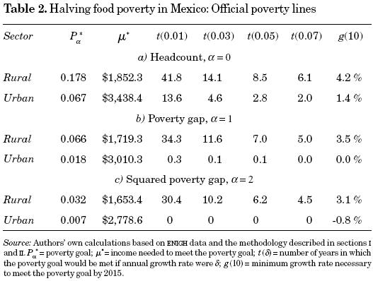
Additionally, using the same methodology, we can compute the minimum necessary growth rate and required number of years needed to halve food poverty intensity in both rural and urban areas. These results are shown in panels b and c of table 2. They show that per capita income in rural areas must grow at least at 3.5 per cent per year to achieve the goal if the poverty gap is considered, and it must grow at 3.1 per cent annually if intensity is measured by the squared poverty gap. Also, the necessary number of years required to attain the objective ranges from 4.5 to 34.3; the more optimistic situation (growth rate of 7 per cent) implies that the goal would be met in less than 5 years, and the more pessimistic (growth rate of 1 per cent) predicts that it would be met in more than 30 years. If we consider the fact that the average growth rate of the primary sector has been around 1.66 per cent since 1980, and that per capita incomes in rural areas have been practically stagnant in the last years, meeting the goals for rural areas seems to be very unlikely.

The urban area represents a completely different situation. The average income in August 2005 is just below the required income to halve poverty intensity –measured by the poverty gap; therefore, the necessary growth rate in the next ten years is close to zero. Also, the time period to attain the goal is less than one year, even if we assume an annual growth rate of 1 per cent. Moreover, the necessary growth rate and number of years to halve poverty intensity –measured by the squared poverty gap–are estimated to be negative, because the required income in 2015 is less than the one registered in August 2005.

The simulations formulated so far should be taken with caution, since the methodology assumes distributional neutral growth. It may be argued that some processes such as migration from rural to urban areas or from Mexico to the United States, and other forms of mobility between formal and informal sectors or among the different economic activities, or differences in growth by sector, may alter the observed income distribution of the reference year (2005) and therefore affect our results.

Finally, using the methodology described in section I.1 we can generate diverse inequality scenarios –inequality measured by the Gini coefficient–to calculate the annual growth rate and the time period required to reduce by half poverty incidence by 2015.⁹ The empirical application is carried out for Gini coefficient values ranging from 0.40 to 0.70.^{10 11}

Figure 1 shows the needed average growth rate between 2005 and 2015 to attain the goal for different Gini coefficient values. Intuitively, the worse the income distribution in 2015, the greater the required growth rate to reach the objective. One can conclude that if the Gini coefficient were below 0.53 by 2015, it would be possible to achieve the goal even if the economy were stagnant. However, if the Gini coefficient were above 0.53, a positive average growth rate would be needed.

Figure 2 shows the year in which this goal would be met if the country grew at different average growth rates (1, 2, 3 and 5 per cent), assuming different income distribution scenarios in 2015. For instance, if the current income distribution holds, then a growth rate as low as would be enough to attain the target.¹²

 

III. Conclusions

We have developed a methodology to analyze the feasibility of reaching different poverty goals under different growth and income distribution scenarios. This methodology considers the entire income distribution, and can be applied to most poverty measures.

Our calculations show that halving poverty incidence and poverty intensity seems to be a plausible event in urban areas, as they only have to grow at rates around 1 per cent per year to achieve the objective by 2015. Nevertheless, accomplishing it in rural areas would require little less than a miracle –assuming that their growth performance in the past continues during the next 10 years.

Public policies have mitigated poverty in rural areas through cash transfer programs, such as "Oportunidades" and "Procampo". They have been effective in increasing the income of poor people living in these areas. However, these programs may not be sufficient to halve poverty by 2015. A more effective and sustainable solution to achieve the MDG, or any other poverty goal, must generate the development of the economic activities associated to the rural sector.

 

References

Aitchison, J. and J. Brown (1966), The Lognormal Distribution, Cambridge University Press.         [ Links ]

Besley, T. and R. Burgess (2003), "Halving Global Poverty", Journal of Economic Perspectives, 17(3), pp. 3–22.         [ Links ]

Bourguignon, F. (2002), "The Growth Elasticity of Poverty Reduction: Explaining Heterogeneity Across Countries and Time Periods", discussion paper.         [ Links ]

Chen, S. and M. Ravallion (2004), "How Have the World's Poorest Fared Since the Early 1980s?", Policy Research Working Paper Series 3341, The World Bank.         [ Links ]

Datt, G. (1998), Computational Tools for Poverty Measurement and Analysis", discussion paper.         [ Links ]

–––––––––– and M. Ravallion (1992), "Growth and Redistribution Components of Changes in Poverty Measures : A Decomposition with Applications to Brazil and India in the 1980s", Journal of Development Economics, 38(2), pp. 275–295.         [ Links ]

Deaton, A. (2003), How to Monitor Poverty for the Millennium Development Goals", Journal of Human Development, 4(3), pp. 353–378.         [ Links ]

ECLAC (2002), "Meeting the Millennium Poverty Reduction Targets in Latin America and the Caribbean", Policy Research Working Paper Series 70, Economic Commission for Latin America and the Caribbean.         [ Links ]

Foster, J., J. Greer and E. Thorbecke (1984), "A Class of Decomposable Poverty Measures", Econometrica, 52(3), pp. 761–766.         [ Links ]

Gastwirth, J. L. (1971), "A General Definition of the Lorenz Curve," Econometrica, 39(6), pp. 1037–1039.         [ Links ]

Hernández L., E. (2005), "Escenarios de la pobreza ante el desarrollo demográfico y económico de México," in CONAPO, México ante los desafíos de desarrollo del milenio, pp. 19–77.         [ Links ]

Kraay, A. (2006), "When is Growth Pro–poor? Evidence from a Panel of Countries", Journal of Development Economics, 80(1), pp. 198–227.         [ Links ]

Li, H., L. Squire and H. Zou (1998), Explaining International and Intertemporal Variations in Income Inequality", Economic Journal, 108(446), pp. 26–43.         [ Links ]

López, H. and L. Servén (2006), "A Normal Relationship? Poverty, Growth and Inequality", Policy Research Working Paper Series 3814, The World Bank.         [ Links ]

Presidencia (2005), "Los objetivos de desarrollo del milenio en México: Informe de avance 2005", discussion paper.         [ Links ]

Ravallion, M. (2001), "Growth, Inequality and Poverty: Looking beyond Averages", World Development, 29(11), pp. 1803–1815.         [ Links ]

–––––––––– and M. Huppi (1989), "Poverty and Undernutrition in Indonesia During the 1980s", Policy Research Working Paper Series 286, The World Bank.         [ Links ]

Villaseñor, J. and B. C. Arnold (1989), "Elliptical Lorenz Curves", Journal of Econometrics, 40(2), pp. 327–338.         [ Links ]

 

Notas

¹ 1) Erradicate extreme poverty and hunger; 2) universal primary education; 3) gender equality; 4) reduce child mortality; 5) improve maternal health; 6) combat hiv/aids and other diseases; 7) environmental sustainability; and 8) develop a global partnership for development. For a more complete description of these goals see www.developmentgoals.org.

² The relative importance of both growth and inequality for poverty is well documented in Datt and Ravallion (1992), Li, Squire and Zou (1998), and Ravallion (2001).

³ To obtain this expression we have used the fact that L'(p)μ = F^–1 (p) (Gastwirth, 1971).

⁴ L (p; π) represents a valid Lorenz curve if, and only if, L (0, π) = 0, L (1, π) = 1, L' (0⁺, π), ≥ 0, and L (p, π) ≥ 0 in p (0,1). For Elliptical Lorenz curves these conditions are equivalent to α< 0, e < 0, d ≥ 0 and a + d ≤ 1 (Villaseñor and Arnold, 1989). For the present application, these criteria were satisfied.

⁵ See Datt (1998) and Villaseñor and Arnold (1989) for details.

⁶ The World Bank has updated this poverty line to 1.08 ppp. This corresponds to a monthly poverty line of 300.6 constant pesos of August 2005.

⁷ Through the empirical analysis, all quantities are set in constant pesos of August 2005.

⁸ Given that a negative number makes no sense, we place a zero to indicate that the goal has already been met.

⁹ For this application we consider a two dollar a day poverty line, given that the one dollar a day line set by the World Bank makes sense only for poorer countries. Previously, the analysis had been carried out for rural and urban areas, but in this section it is performed at the national level; therefore, one dollar a day represents a low target.

¹⁰ In the case of Mexico, the Gini coefficient has fluctuated between 0.50 and 0.55 in the past.

¹¹ Evidence in favor of the lognormality of income assumption is shown in the Appendix.

¹² Hernández L. (2005) presents a similar empirical application (assumes different growth rates and different levels of income inequality). Nevertheless, our results are not fully comparable given that we use a different poverty line, a different reference year, and we focus on analyzing the necessary growth rates to halve poverty by 2015. A closely related document by ECLAC (2002) estimates isopoverty curves to analyze several distribution and growth scenarios to halve poverty by 2015 for several Latin American countries. However, the results of this study are not fully comparable to ours either, since they use 1999 as the reference year.

¹³ An Epanechnikov Kernel with bandwidth .3 was used in this application.