Statistical models

(Equation 1) is the model used under the GBLUP model. Where represents the normal response observed in the -th line in the j-th environment, where i=1,2,…1I;j=1,2,…J.

Note that E _i represents the j-th environment, G represents the genomic effect of the j-th line and is assumed as a random effect distributed as G=(G1,…,Gj )T∼N(0,G1 σG2), where G ₁ denotes the genomic relationship matrix calculated as suggested by ^{Van (2008)} and σG2 denotes the genomic variance. On the other hand EG _ij is the interaction between the genomic effect of the j-line with the i-th environment and is also assumed as a random effect distributed as G=(EG11,… ,EGIJ )T∼N(0,G1⨂ II σGE2), where σGE2 denotes the variance of the interaction of genotype by environments. Finally, ε _ij is the random error term associated with the j-th line in the i-th environment distributed N(0,σGE2), where σe2 denotes the residual variance.

On the other hand, to make the prediction of all traits simultaneously we propose the model given in equation (2),

Where y _ijk is the response variable in the i-th environment, j-th line and k-th trait, ET _ik represents an interaction between the i-th environment and k-th trait, GT _jk represents an interaction between the genomic effect of the j-th line and the k-th trait and is assumed as a random effect TG=(TG11,…,TGJI)T∼N(O,G1⨂IkσGT2) where σGT2 denotes the variance of the interaction of genotype by trait. EGTijkrepresents the triple interaction between the i-th environment, j-th line and k-th trait and is assumed as a random effect, and is distributed as ETG=(ETG111,…,ETGIJI)T∼N(0,II⨂G1⨂Ik σEGT2 ), where σEGT2 denotes the variance of the three way interaction, while ε _ijk is a random error term corresponding to the i-th environment, j-th line and k-th trait, and is assumed to be distributed N(0,σε2), where σε2 denotes the residual variance. It is important to mention that the implementation of the model given in (equation 1) was done using the GFR package provided in the publication of ^{Montesinos-López et al. (2018)} while the second model given in (equation 2) was implemented in the R package BGLR ^{(de los Campos and Pérez-Rodríguez, 2016)}. We performed a total of 20,000 iterations; 5,000 samples were used for inference because the first 15,000 were used as burn-in to decrease the MCMC errors in prediction accuracy.

Item based collaborative filtering (IBCF)

The IBCF algorithm is very popular with electronic-commerce web sites for recommending items and products, where they use inputs about a customer’s interests to generate a list of recommended items. This algorithm was recently implemented in genomic selection and proved to be comparable to conventional whole- genome prediction models when the correlation between traits and environments was moderate or high (^{Montesinos-López et al., 2018}). The IBCF algorithm works by building a database of users’ (lines) preferences for items (trait-environment combination). For example, Table 1a provides raw phenotypic data with six lines evaluated in two different environments (E1 and E2) for two different traits (T1 and T2) with both traits in different scales, also this raw phenotypic data set has 4 missing values (with NA). Then we standardize by column ([zij=(yij-μj)σj1)] each column of Table 1a (except the first one), where i denotes the users (lines) and j denotes the columns (trait-environment combinations), and we form the standardized information in Table 1b. In this example i =1,…,6, j =1,2…,4, μ _j , is the mean of column j and σ _j denotes the standard deviation of column j. Also, for comparison purposes we know that the true values for the missing values are: y ₂₁ =14.0971, y ₃₄ =5.3511, y ₄₂ =8.9786 and y ₅₃ =8.2019 respectivelly. Then we calculated the Pearson correlation between Table 1b columns (trait-environment combinations) shown in Table 1c. Next with the following formula, we calculate the predictions for the missing phenotypes of line i in item j (Sarwar et al., 2001; ^{Montesinos-López et al., 2018}).

Where ẑij,=∑j'ϵNijzij'wjj'∑j'ϵNij|wjj'| is the predicted scaled phenotype for user (line) i on ítem (trait-environment) j. N _i (j) denotes the items rated by user (line) i most similar to item j, w_jj is the weight between items j and j´ and the weights used in formula (3) are obtained from an item-to -item similarity matrix built using the Pearson’s correlation (Given in Table 1c), which provides information on how similar an item is to another item.

Next, we illustrate how to calculate the four missing values using formula (1). First, we calculate the scaled predicted value for y ₂₁

Then the predicted value of y₂₁ in its original scale is equal to

This mean that the predicted value of line 2 in trait-environment combination 1(y^21) is 14.0408 wich is close to the true value 14.0971. Next, we show how to calculate the predicted value for the missing value y^34; first the scaled predicted values are equal to

Then the predicted value of y ₃₄ in its original scale is equal to

Now the predicted value of line 3 in trait-environment combination 4 (y^34) is 4.8146 wich is close to the true value 5.3511. Then, we present the scaled predicted response for line 4 and trait-environment combination 2, y ₄₂ , which is

Then the predicted value of y ₄₂ in its original scale is equal to

This mean that the predicted value of line 4 in trait-environment combination 2 (y^42) is 10.0673 wich is close to the true value 8.9786. Finally, we present the scaled predicted value of line 5 in the trait-environment combination 3,

Then the predicted value of y ₅₃ in its original scale is equal to

This mean that the predicted value of line 5 in trait-environment combination 3 (y^53) is 7.9237 wich is close to the true value 8.2019.

As we can see with this example the calculations are easy but laborious, but the IBCF.MTME packages do this job automatically and the data set required can be on different scales (not standardized) for the traits, that is, the traits are allows to be measured on different scales. Internally, the IBCF. MTME package standardize ([zij=(yij-μj)σj-1]) each column of the data set given in Table 2 (that shows the format of the type of data required) for the training data set obtained in each random partition. This implies that to use the formula given in (equation 3) for making predictions about trait-environment combinations, after standardizing is calculated the similarity matrix resulting from the corresponding training data set of a partition selected from the whole data set in Table 2. Therefore, the predictions obtained by using (equation 3) with the parameters estimates required obtained with the training data set corresponding to each partition and the predictions are done for the observations in testing data set.

Evaluation of the prediction accuracy

Two cross-validation schemes were used to assess the prediction accuracy of both models. Both schemes simulate two key situations that breeders often witness. The first corresponds to a cross validation with 10 random partitions, which simulates situations where some lines have been evaluated in some environments but in others are lost. The percentage of missing values correspond to 20% of the lines of each data set, in other words, 80% of the observations in the data sets have been used to train the models.

The second scheme simulates a situation with a non-evaluable trait in all the lines in an environment, but is present in the remaining environments. In this case, information from known data in other environments is used, and the evaluation of the prediction can benefit from the loan of information between lines across environments, and between correlated traits. From the variety of methods used to compare the predictive ability, we used Pearson´s correlation and we report the average of the 10 random partitions. Models with a higher correlation indicate better predictions.

Statistical software

The statistical software R version 3.5.0 (^{R Core Team, 2018}), was used using the external packages IBCF.MTME version 1.2-5 and the GFR package which includes different tools that provide some points for prediction models implementation in the GS context, this package was used in version 0.9-12 (^{Montesinos-López et al., 2018}).

Real data sets

This research analyzed six different real datasets obtained from various studies, the data are available in the following link, below is a description of the content of each data set.

Maize dataset

This data set is based on that of ^{Montesinos-López et al. (2017)}. It is composed of a sample of 309 maize lines evaluated for three traits: anthesis-silking interval (ASI), plant height (PH), grain yield (GY), each of them evaluated in three optimal storm environments (Env1, Env2 and Env3). The total number of genomes by sequencing (GBS) data were 681,257 single nucleotide polymorphisms (SNPs), and, after filtering for missing values and minor allele frequency, were used 158,281 SNPs for the analyses. We have identified this data set as Maize. For more details, see the study of ^{Montesinos-López et al. (2017)}.

Maize Hel dataset

This data set is based on the data used in the study of ^{Cuevas et al. (2018)}. It consists of a sample of 247 maize lines evaluated in 2015 in three environments corresponding to Nova Mutum (NM) in the state of Mato Grosso, Pato de Minas (PM) and Ipiaçú (IP) in the state of Minas Gerais, Brazil. The traits evaluated were: Ear height (EH), PH and GY. The HEL parent lines were genotyped with an Affymetrix Axiom Maize Genotyping Array of 616 K SNPs with standard quality controls removing markers with a Call Rate 0.95. This data set differs from the cited study is the elimination of unmeasured maize lines in one of the traits, as well as two environments where the three traits had not been measured in an effort to have a balanced data set, in the same way they were removed from the genomic matrix. We have identified this data set as Maize_HEL. For more details, see the study of ^{Cuevas et al. (2018)}.

Maize USP dataset

This data set is based on the data used in the study of ^{Cuevas et al. (2018)}. It consists of 720 lines of corn evaluated in Piracicaba and Anhumas, Brazil, each with two levels of nitrogen fertilization (N): Ideal N (IN) and Low N (LN) for a total of four artificial environments (PIN, PLN, AIN and ALN), for three traits (EH, PH, GY). Like the data set Maize_HEL, the Maize_USP parent lines were genotyped with an Affymetrix Axiom Maize Genotyping Array of 616 K SNPs with standard quality controls removing markers with a Call Rate 0.95 in addition. Like the above data set, it differs from the data from the cited study in the removal of lines that did not contain all its complete measurements to have a balanced data set. We have identified this data set as Maize_USP. For more details, see the study of ^{Cuevas et al. (2018)}.

Wheat BGLR dataset

This data set is based on the data used in the study of ^{Crossa et al. (2010)} and it is preloaded in the BGLR package. It consists of 599 wheat lines evaluated in four different environments. The 599 wheat lines were genotyped using 1447 Diversity Array Technology (DArT) markers. The markers with a minor allele frequency (MAF) (0.05) were removed, and missing genotypes were imputed using samples from the marginal distribution of marker genotypes. The number of DArT markers after edition was 1279. We have identified this data set as Wheat_BGLR. For more details, see the study of ^{Crossa et al. (2010)}.

Wheat IBCF dataset

This data set is based on the data used in the study of ^{Montesinos-López et al. (2016)} a multi-environment single trait model for assessing genotype \u00d7 environment interaction (G \u00d7 E and it is preloaded in the IBCF.MTME package. It consists of a sample of 250 lines of wheat grown during the 2013-2014 harvest season in Ciudad Obregon, Sonora, Mexico. The trials were planted in mid-November and grown in beds with 5 and 2 irrigations plus drip irrigation. Four traits were recorded: (1) Days to heading (DT) which corresponds to the number of days from germination until 50% of the peaks in each plot appeared, (2) GY corresponding to the total grain yield of the plot after maturity, (3) PH recorded in centimeters, and (4) the vegetative index (NDVI) was calculated from the data collected through a hyperspectral chamber. Genotyping-by-sequencing was used for genome-wide genotyping. Single nucleotide polymorphisms were called across all lines using the TASSEL GBS pipeline anchored to the genome assembly of Chinese Spring. Single nucleotide polymorphism calls were extracted, and markers filtered so that percent missing data did not exceed 80% and 20%, respectively. Individuals with 80% of missing marker data were removed, and markers were recorded as 2, 0, and 1, indicating homozygous for the minor allele, heterozygous, and homozygous for the major allele, respectively. Next, markers with 0.01 minor allele frequency were removed, and missing data imputed with the marker mean. A total of 12,083 markers remained after marker editing. We have identified this data set as Wheat_IBCF. For more details, see the study of ^{Montesinos-López et al. (2016)} a multi-environment single trait model for assessing genotype \u00d7 environment interaction.

Wheat Iranian dataset

This data set is based on the data used in the study of ^{Crossa et al. (2016)}. It consists of 2374 wheat lines that were evaluated in field (D) and heat (H) drought experiments at the CIMMYT experimental station near Ciudad Obregón, Sonora, Mexico (27°20′ N, 109°54′ W, 38 meters above sea level), during the Obregón 2010-2011 cycle. Two traits were evaluated (DTM days at maturity and DTH days to heading). From a total of 40,000 markers, after quality control 39,758 markers were used. We have identified this data set as Wheat_Iranian. For more details, see the study of (^{Crossa et al., 2016}).

Maize dataset

Figure 1 shows two types of predictions using the two implemented models GBLUP and IBCF. First, the predictions are presented using the breeding values (phenotypic values adjusted using the markers) and these are the values that will be predicted. In the second case, the goal is to predict the phenotypic values. Under the GBLUP model, two models are fitted with genomic information and without the genomic information.

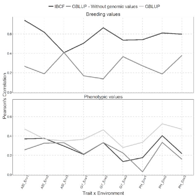
Figure 1 Prediction accuracy of CV1 obtained with Pearson´s correlation for both models IBCF and GBLUP, using phenotypic values and breeding values as the response variable for the Maize data set. The results of average Pearson´s correlation correspond to the testing set of a cross validation with 10 random partitions with 80% for training and 20% for testing
Figura 1. Capacidad predictiva de CV1 obtenida con la correlación de Pearson para ambos modelos IBCF y GBLUP, utilizando valores fenotípicos y valores genéticos como variable respuesta para el conjunto de datos de Maize. Los resultados de la correlación promedio de Pearson corresponden al conjunto de prueba de una validación cruzada con 10 particiones aleatorias con 80% para entrenamiento y 20% para prueba. 

The best predictions are observed under the scenario for breeding values compared with that for phenotypic values, which is to be expected, since it eliminates the uncertainty by the adjustment to the phenotypic values by the markers to obtain the breeding values. When breeding values are predicted, it is observed that the best predictions in most of the trait-environment combinations have been obtained through the IBCF model, because when comparing these results with the GBLUP model, differences can be appreciated in most cases (8 out of 9 trait-environment combinations). Only in the trait-environment ASI-Env3 is similar between the predictive capabilities of both models, the rest of the combinations IBCF model is superior to GBLUP (Figure 1).

On the other hand, when using phenotypic values, we can observe similar results between IBCF and GBLUP without the genetic values. The GBLUP obtains significantly lower predictive capacities only in two points and these correspond to the ASI and PH traits for environment 1. When comparing the GBLUP with genetic values versus the IBCF, we found that 7 out of 9 trait-environment combinations are different and GBLUP shows better prediction accuracy (Figure 1).

Figure 2 show the same two types of cross-validation given in Figure 1. However, now the predictions were made for all lines of one environment for each trait, using the remaining data as training data (CV2).

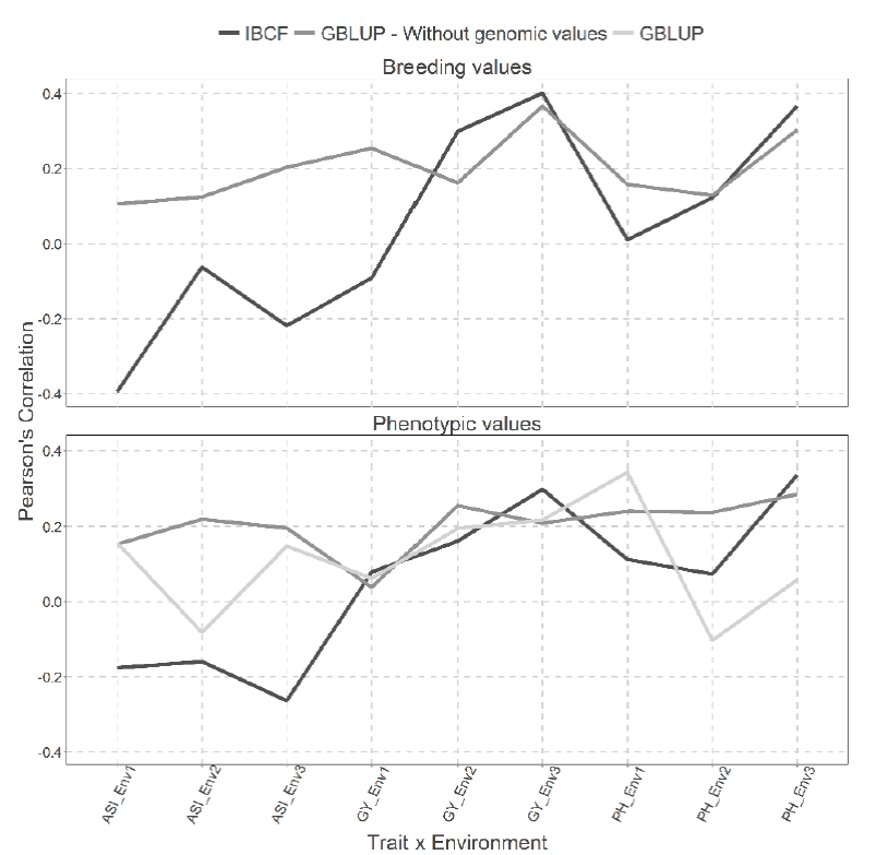
Figure 2 Predictive accuracy of CV2 obtained with Pearson´s correlation for the two models IBCF and GBLUP, using phenotypic values and breeding values as the response variable for the Maize data set. Pearson´s correlation are reported for each trait-environment combination
Figura 2. Capacidad predictiva de CV2 obtenida con la correlación de Pearson para los dos modelos IBCF y GBLUP, utilizando valores fenotípicos y valores geneticos como variable de respuesta para el conjunto de datos de Maize. La correlación de Pearson se informa para cada combinación de rasgo-ambiente. 

When predicting breeding values, the GBLUP model proved to be superior. In ASI trait in all environments, we obtained the best predictions under the GBLUP model. While in GY trait, the best predictions were observed only in the first environment, while in the remaining environments the best predictions were observed under the IBCF model (Figure 2).

On the other hand, using phenotypic values, we observe that using the GBLUP model without genetic values results in better predictions for the ASI trait in the three environments and for the PH trait in environments 2. While including the genetic values gives better predictions only for PH trait in environment 1 (Figure 2).

Finally, we compared the runtimes of GBLUP vs. IBCF for Maize data using the breeding values and found that the GBLUP takes 35.48 seconds to implement while the IBCF takes only 2.5 seconds, which means that the IBCF is 14.19 times faster than the GBLUP model (Table 2).

Maize HEL dataset

Figure 3 show two types of predictions for both type of models under CV1 cross validation, the first for predicting the breeding values and the second for predicting the phenotypic values. We cannot observe gain between the scenarios where breeding values have been predicted against the scenarios where phenotypic values were predicted for the Maize_HEL data set. When the breeding values were predicted the results obtained are quite similar (2 of 9 combinations are different) under both models, with the exception for the GY trait in the IP and PM environments, where the best predictions accuracies were obtained by the IBCF model (Figure 3).

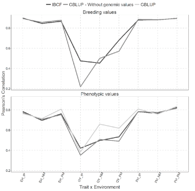
Figure 3 Prediction accuracy under CV1 with Pearson´s correlation for models IBCF and GBLUP, using phenotypic values and breeding values as the response variable for the Maize_HEL data set. The results of average Pearson correlation correspond to a cross validation with 10 partitions with 80 % for training and 20% of testing.
Figura 3. Capacidad predictiva bajo CV1 con la correlación de Pearson para los modelos IBCF y GBLUP, utilizando valores fenotípicos y valores genéticos como variable respuesta para el conjunto de datos Maize_HEL. Los resultados de la correlación promedio de Pearson corresponden a una validación cruzada con 10 particiones con 80% para entrenamiento y 20% de prueba. 

We can observe for the analysis performed using the phenotypic values, that the results obtained with the GBLUP model with (and without) the genomic values are similar to the results obtained with the IBCF model (only 1 out of 9 combination is different) this difference was obtained for the GY trait in the NM environment (Figure 3).

Figure 4 also give the same two types of predictions than in Figure 3, but implemented with the CV2 cross validation. Better predictions were obtained under the scenario where breeding values were predicted than under the scenario where phenotypic values were predicted. When breeding values were predicted, small differences were observed between both models, except in the trait-environment combination that corresponds to the GY trait in the IP environment where the best predictions were under the IBCF model. On the other hand, for the three trait-environment combinations that correspond to the PH the best predictions were observed with the GBLUP model (Figure 4).

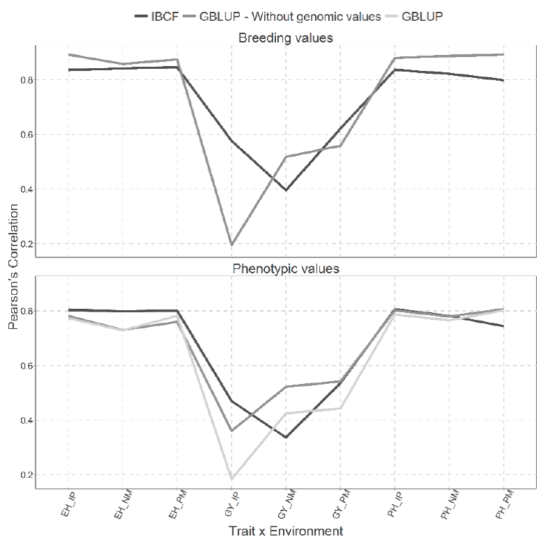
Figure 4 Prediction accuracy under CV2 with Pearson´s correlation for two models IBCF and GBLUP, using phenotypic values and breeding values as the response variable for the Maize_HEL data set. Pearson´s correlation results correspond to each trait-environment combination
Figura 4. Capacidad predictiva bajo CV2 con la correlación de Pearson para dos modelos IBCF y GBLUP, utilizando valores fenotípicos y valores genéticos como variable respuesta para el conjunto de datos Maize_HEL. Los resultados de la correlación de 

When the phenotypic values were predicted, the results obtained with the GBLUP model without using the genotypic values are similar to those obtained with the IBCF model, although in the trait-environment combination GY-NM, lower predictions were obtained with the IBCF model. Finally, with the GBLUP model with genomic information we observed low predictions for the GY trait for the environments IP and PM (Figure 4).

Finally, we compared the runtimes of GBLUP versus IBCF for the Maize_HEL data set using the breeding values and we found that the GBLUP takes 31.23 seconds to implement while the IBCF takes only 0.79 seconds, which means

Figure 6, as Figure 5, also shows two types of predictions with breeding values and phenotypic values, but with the cross validation, CV2. We obtained better predictions under the scenario predicting breeding values, than under the scenario where phenotypic values are predicted. When predicting breeding values, we observed the best predictions under the GBLUP model for all the trait-environment combinations.

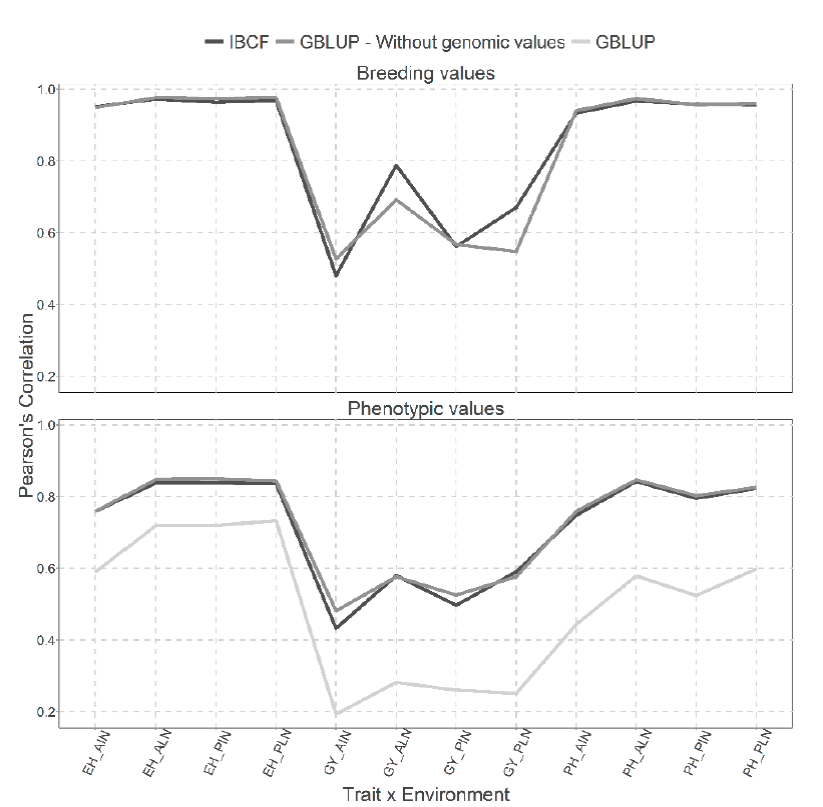
Figure 5 Prediction accuracy under CV1 with Pearson´s correlation for models IBCF and GBLUP, using phenotypic values and breeding values as the response variable for the Maize_USP data set. The results of average Pearson´s correlation correspond to a cross validation with 10 partitions with 80 % for training and 20% of testing
Figura 5. Capacidad predictiva bajo CV1 con la correlación de Pearson para los modelos IBCF y GBLUP, utilizando valores fenotípicos y valores genéticos como variable respuesta para el conjunto de datos Maize_USP. Los resultados de la correlación promedio de Pearson corresponden a una validación cruzada con 10 particiones con 80% para entrenamiento y 20% de prueba 

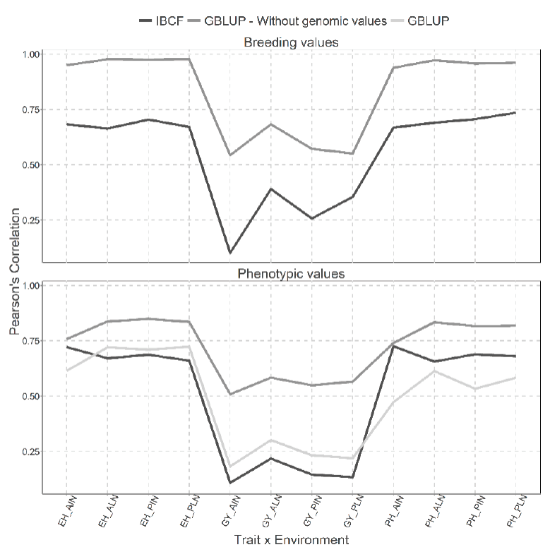
Figure 6 Prediction accuracy under CV2 with Pearson´s correlation for two models IBCF and GBLUP, using phenotypic values and breeding values as the response variable for the Maize_USP data set. Pearson´s correlation results correspond to each trait-environment combination.
Figura 6. Capacidad predictiva bajo CV2 con la correlación de Pearson para dos modelos IBCF y GBLUP, utilizando valores fenotípicos y valores genéticos como variable respuesta para el conjunto de datos Maize_USP. Los resultados de la correlación de Pearson corresponden a cada combinación de rasgo-ambiente. 

On the other hand, for the results predicting the phenotypic values, we observe similar results with the IBCF and GBLUP models that takes into account the genomic values, except in some points where the IBCF had deficiencies. These correspond to the GY trait for all the environments, as well as some points where it has obtained better predictive capacities; these correspond to the PH trait for all the environments. However, when the genomic values were removed from the GBLUP model, was the best for all the trait-environment combinations.

Finally, we compared the runtimes of GBLUP versus IBCF for the Maize_USP data set with breeding values and we found that the GBLUP takes 275.58 seconds to implement while the IBCF takes only 2.95 seconds, which is equivalent to the IBCF being 93.42 times faster than the GBLUP model (Table 2).

Maize USP dataset

Figure 5 presents under CV1 cross validation, two types of predictions for both type of models, the first for predicting the breeding values and the second for predicting the phenotypic values. We can observe a gain in the scenario where breeding values have been predicted against the scenarios where phenotypic values were predicted for the Maize_USP data set. When the breeding values were predicted, the results obtained are quite similar (9 of 12 combinations are similar) and of those different two of them favor the IBCF model and one the GBLUP model (Figure 5). While for the analysis performed using the phenotypic values, it is evident that the results obtained with the IBCF and GBLUP model without the genomic values are better to the results obtained with GBLUP model with the genomic values. However, the GBLUP model without the genomic values are similar to the results obtained with the IBCF model (Figure 5).

Wheat BGLR dataset

Figure 7 shows two types of predictions for both type of models, under CV1 cross validation. The best predictions were under the scenario that predicts the breeding values compared with the scenario that predicts the phenotypic values for the Wheat_BGLR data set. When the breeding values were predicted, it is observed that the IBCF was better in 3 out of 4 combinations than the GBLUP (Figure 7). On the other hand, when using the phenotypic values, it is evident that the GBLUP model without genomic information is quite similar to the IBCF model. While the for the GBLUP model with the genomic information produced the lower predictions (Figure 7)

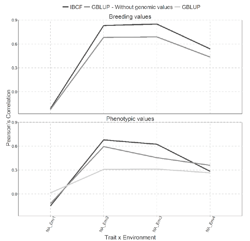
Figure 7 Prediction accuracy under CV1 with Pearson´s correlation for models IBCF and GBLUP, using phenotypic values and breeding values as the response variable for the Wheat_BGLR data set. The results of average Pearson correlation correspond to a cross validation with 10 partitions with 80 % for training and 20% of testing.
Figura 7. Capacidad predictiva bajo CV1 con la correlación de Pearson para los modelos IBCF y GBLUP, utilizando valores fenotípicos y valores genéticos como variable respuesta para el conjunto de datos Wheat_BGLR. Los resultados de la correlación promedio de Pearson corresponden a una validación cruzada con 10 particiones con 80% para entrenamiento y 20% de prueba. 

Finally, we compared the runtimes for the GBLUP versus the IBCF for the Wheat_BGLR data using the breeding values and we found that the GBLUP takes 197.82 seconds to implement, while the IBCF takes only 0.66 seconds, which means that the IBCF is 299.73 times faster than the GBLUP model (Table 2).

Wheat IBCF dataset

Figure 8 presents two types of predictions for both type of models, the first for predicting the breeding values and the second for predicting the phenotypic values. For these cases, CV1 cross validation has been used.

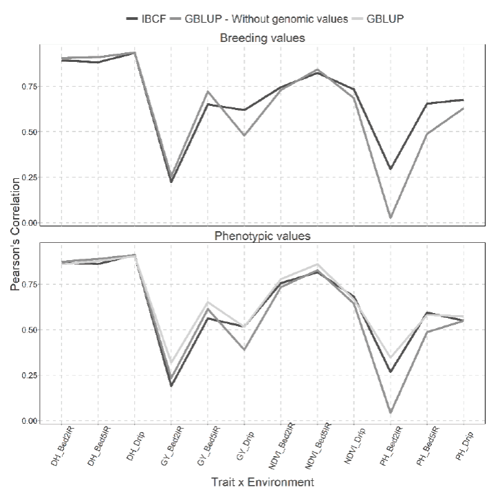
Figure 8 Prediction accuracy under CV1 with Pearson´s correlation for models IBCF and GBLUP, using phenotypic values and breeding values as the response variable for the Wheat_IBCF data set. The results of average Pearson´s correlation correspond to a cross validation with 10 partitions with 80 % for training and 20% of testing
Figura 8. Capacidad predictiva bajo CV1 con la correlación de Pearson para los modelos IBCF y GBLUP, utilizando valores fenotípicos y valores genéticos como variable respuesta para el conjunto de datos Wheat_IBCF. Los resultados de la correlación promedio de Pearson corresponden a una validación cruzada con 10 particiones con 80% para entrenamiento y 20% de prueba. 

When the breeding values were predicted, it is observed that the models obtain similar predictions because only 4 of 12 combinations are different and three of them result in better predictions for the IBCF model, this correspond to PH trait in the Bed2IR and Bed5IR environments and GY trait in the Drip environment. In addition, the remaining combination corresponds to GY trait in Bed5IR environment that result in better prediction for the GBLUP model (Figure 8).

Meanwhile for the analysis performed using the phenotypic values, we can observe that in general the GBLUP without using the genomic information was the worst in terms of prediction performance than the other two methods (IBCF and GBLUB with genomic information) (Figure 8).

Two types of predictions using the two models GBLUP and IBCF are presented in Figure 9 with breeding values and phenotypic values, but with the cross validation, CV2. When predicting breeding values, remarkable differences are observed between both models, it is observed that under the GLBUP the best predictions were observed for traits DH and GY, while under the IBCF method the best predictions were observed under trait NDVI (Figure 9). While, for the results obtained when using the phenotypic values, we observe the same pattern, but the GBLUP model with or without genetic information produced similar predictive capacities (Figure 9).

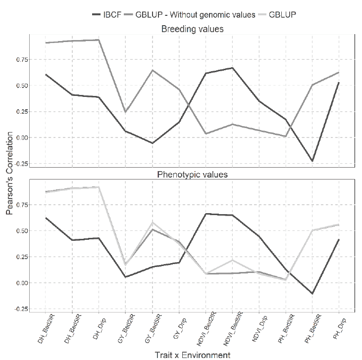
Figure 9 Prediction accuracy under CV2 with Pearson´s correlation for two models IBCF and GBLUP, using phenotypic values and breeding values as the response variable for the Wheat_IBCF data set. Pearson´s correlation results correspond to each trait-environment combination.
Figura 9. Capacidad predictiva bajo CV2 con la correlación de Pearson para dos modelos IBCF y GBLUP, utilizando valores fenotípicos y valores genéticos como variable respuesta para el conjunto de datos Wheat_ IBCF. Los resultados de correlación de Pearson corresponden a cada combinación de rasgo-ambiente. 

Finally, we compared the runtimes for the GBLUP vs. IBCF for Wheat_IBCF data using the breeding values and we found that the GBLUP takes 34.28 seconds to implement while the IBCF takes only 1.03 seconds, which means that the IBCF is 33.28 times faster than the GBLUP model (Table 2).

Figura 7

Wheat Iranian dataset

Figure 10 presents two types of predictions for both type of models, the first for predicting the breeding values and the second for predicting the phenotypic values. For these cases, CV1 cross validation has been used.

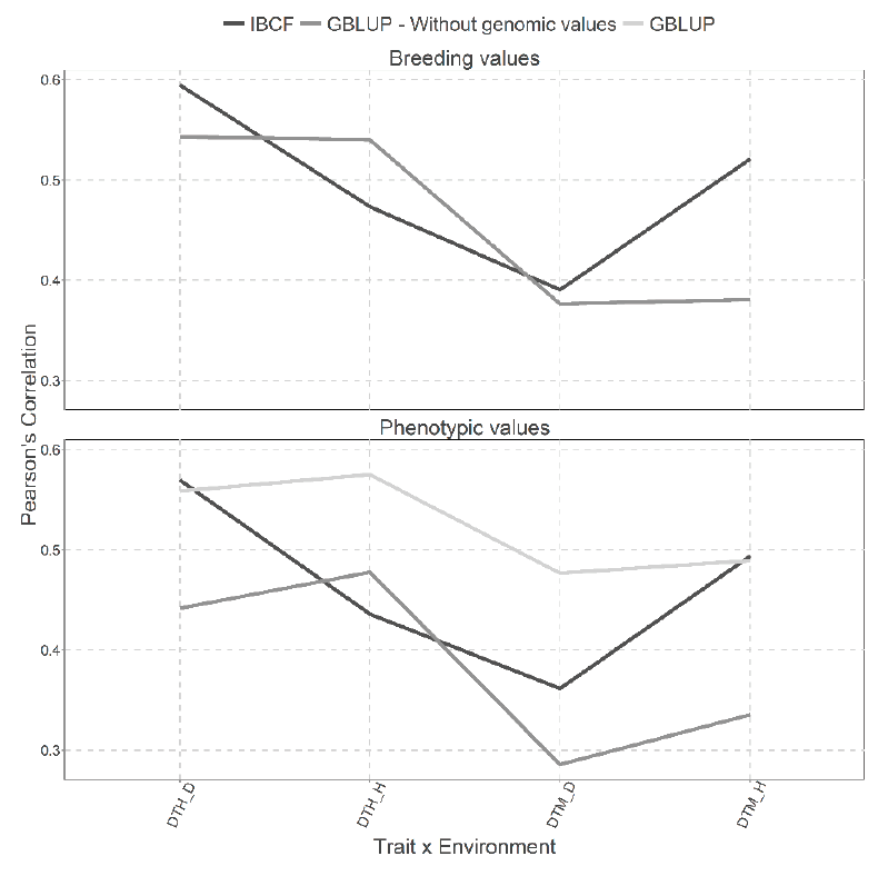
Figure 10 Prediction accuracy under CV1 with Pearson´s correlation for models IBCF and GBLUP, using phenotypic values and breeding values as the response variable for the Wheat_Iranian data set. The results of average Pearson correlation correspond to a cross validation with 10 partitions with 80 % for training and 20% of testing.
Figura 10. Capacidad predictiva bajo CV1 con la correlación de Pearson para los modelos IBCF y GBLUP, utilizando valores fenotípicos y valores genéticos como variable respuesta para el conjunto de datos Wheat_Iranian. Los resultados de la correlación promedio de Pearson corresponden a una validación cruzada con 10 particiones con 80% para entrenamiento y 20% de prueba. 

We can observe little gain between the scenarios when using breeding values against the scenarios using phenotypic values to predict for the Wheat Iranian data set. When the breeding values are predicted, it is observed that no great differences in the predictions between both models because 3 of 4 combinations are quite similar (Figure 10). When using the phenotypic values, it is evident that results obtained with the GBLUP model without the genomic values are better than those obtained with the IBCF model and the GBLUP model with genomic information. However, the IBCF was better than the GBLUP model with genomic information (Figure 10).

Two types of predictions were performed with the GBLUP and IBCF models in Figure 11 with breeding values and phenotypic values, but with the cross validation, CV2. We obtained better predictions under the breeding values scenario. Under predicted breeding values, the results obtained under the IBCF model are higher than those obtained by the GBLUP model in all the traits for all the environments (Figure 11). While, for the results obtained when using phenotypic values, the same pattern is observed, that is the IBCF was the best; however, the GBLUP model without the genetic information was better in prediction accuracy than the GBLUP with genomic information (Figure 11).

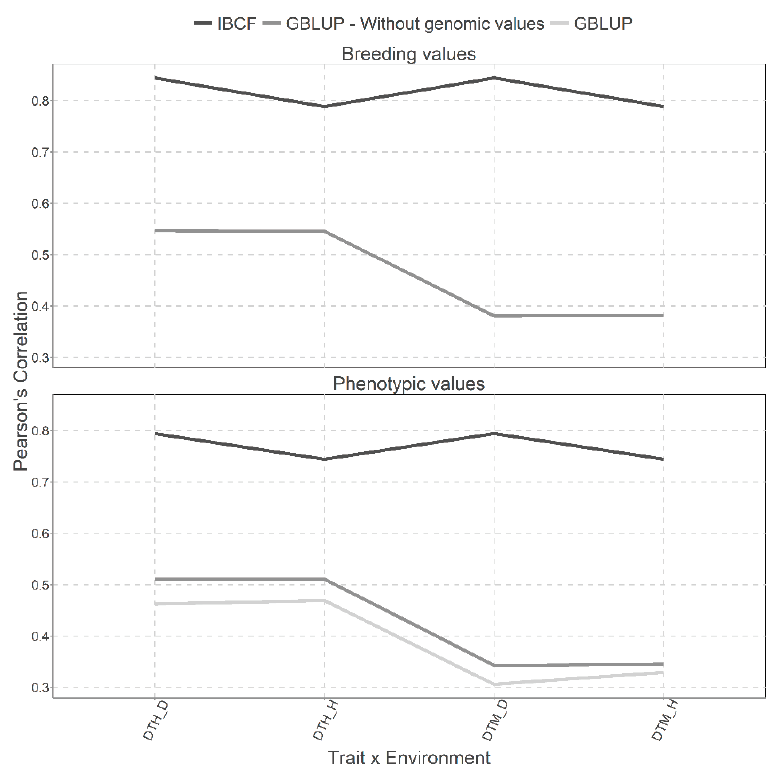
Figure 11 Prediction accuracy under CV2 with Pearson´s correlation for two models IBCF and GBLUP, using phenotypic values and breeding values as the response variable for the Wheat Iranian data set. Pearson´s correlation results correspond to each trait-environment combination
Figura 11. Capacidad predictiva bajo CV2 con la correlación de Pearson para dos modelos IBCF y GBLUP, utilizando valores fenotípicos y valores genéticos como variable respuesta para el conjunto de datos de trigo iraní. Los resultados de la correlación de Pearson corresponden a cada combinación de rasgo-ambiente. 

Finally, we compared the runtimes for the GBLUP vs. IBCF for Wheat_Iranian data using the breeding values and we found that the GBLUP takes 1152.36 seconds to implement while the IBCF takes only 2.19 seconds, which means that the IBCF is 526.19 times faster than the GBLUP model (Table 2).

Time of execution between the models IBCF and GBLUP

Table 2 shows the execution times in seconds implemented by each model, showing that the IBCF model is able to process information more quickly, in the case of the smaller data sets used in this research, as: Maize, Maize_HEL and Wheat_IBCF show a difference ratio between the GBLUP and IBCF models between 15 and 33 times faster, while for the larger data sets used in this research, such as Maize_USP, Wheat_BGLR and Wheat_Iranian, a difference ratio between both models between 93 and 526 times faster is shown.

It is important to note that on average across data sets the GBLUP model requires 286.12 seconds to adjust the model, while IBCF requires only 1.68 seconds on average, that is, the IBCF method is 169.63 times faster than the GBLUP model.