


 nueva página del texto (beta)
 Inglés (pdf)
 Artículo en XML
 Referencias del artículo
 Enviar artículo por email
 Citado por SciELO
  Similares en
SciELO
Similares en
SciELO 
 Permalink
Introduction
Defining city boundaries is likely a problem without solution. This is more noticeable in undeveloped countries, where lack of data at national level makes the definition of urban agglomeration boundaries more problematic. Where do cities end and meet the countryside? How to reveal an urban-like pattern without subjectivity? Is percolation theory useful in showing contiguous metropolitan relationships without the use of origin–destination data? These and other questions arise in this research article by applying percolation theory to the Mexican national road network and comparing its results with the National Urban System (SUN).
In 2016, colleagues from the Centre for Advanced Spatial Analysis (CASA), University College London, found a very promising and interesting relationship between the fractal dimension as obtained through percolation theory, and how the British Urban System is hierarchically arranged (Arcaute et al., 2016). In their work, they used percolation theory over Britain’s road network, establishing hierarchies at different percolation thresholds. Several regions (or clusters) were formed at different distances of the percolations (i.e., several small “patches” emerged when the percolation process was calculated at a very short distance, for instance 10 m, and one single cluster was formed when the percolation process was calculated at the maximum percolation distance). But the most striking revelation was that when computing the fractal dimension of the extracted clusters, they observed that it “reaches a maximum plateau at a specific distance [and that] the clusters defined at this distance threshold are in excellent correspondence with the boundaries of cities recovered from satellite images, and from previous methods using population density” (Arcaute et al., 2016: 1). In other words, they found a threshold at which emergent clusters can be identified as “cities” by analyzing their fractal dimension.
Numerous authors have been using percolation theory to: a) understand if urban growth patterns are correlated with percolation (Makse et al., 1998); and b) to find urban-rural limits which, in the end, define city limits (Cao et al., 2020). The latter improves the referred method (Arcaute et al., 2016) by using multi-source urban data as input for percolation, and by finding maximum thresholds when city-like clusters are formed for additional measures to the fractal dimension, like Shannon’s entropy for road density, population density, and the Digital Number (DN) Value of nightlights data series. But what does this mean?
The goal in this paper is to delve into the findings of percolating the Mexican road network and finding the limits of urban regions, compared to those defined in the SUN, to determine cities’ boundaries in a more automated and less subjective way. The SUN is more suited for public policy rather than understanding urban dynamics because policies are applied at the administrative level. The current SUN definition has some political deviations, uses criteria that may be too subjective or arbitrary, like the inclusion of administrative boundaries of continuous and complete municipalities, or using population as an input to determine the size of an urban area. The SUN is an instrument that allows the federal government to put in place strategies and programs derived from land use policies, and its goal is to be used as a tool to support strategic planning and decision-making in urban scopes and land policy. Therefore, it becomes relevant to delimit urban regions as there are cases of public resources being applied only to urban municipalities.
The method presented here, focuses more on the detail where urban agglomerations tend to end, it does not carry any inherent political implications, aggregates urban dynamics in a reproducible, mathematical form, and uses geographical space as the input where human exchanges take place. As such, it aims to look into the real urban dynamics, as opposed to administrative ones.
In order to better understand this procedure, a brief theoretical frame for understanding the observed relationship between percolation, fractal dimension, and cities is needed.
1. Percolation theory
Percolation is a probability model whose roots can be found in physicsrelated problems since 1957, when two researchers asked themselves what was the probability of the center of a porous stone immersed in a bucket of water getting wet? (Grimmett, 1999: 1). One simple explanation of percolation theory is provided by Stauffer and Aharony (2018). It goes as follows (see figure 1): suppose that in a large square lattice whose boundaries are negligible due its large size, certain squares are filled with dots on their centers while others are left empty. In doing so, we can later observe points closer to others, thus forming clusters. Such clusters are formed when points have at least a neighboring square that has one side in common. Those observed patterns –– in number and properties –– are among the subjects of study of percolation theory. Percolation theory is mainly about the probability of a square being occupied by a dot. As stated by Stauffer and Aharony (2018: 3): “Percolation theory deals with the clusters thus formed, in other words with the groups of neighboring occupied sites”. A large part of percolation theory is devoted to understanding the moment when the first cluster appears. It is called the critical phenomenon or the moment in which the system drastically changes, which in turn could be explained by the scaling theory.
For Arcaute et al., (2016), percolation theory can be extended to finite systems, such as urban agglomerations (traditional percolation theory was originally developed for infinite systems). Central to them is the notion that a system, through different percolation processes, can show hierarchical structures and thus, expose the hierarchical organization of a certain national urban system regardless of its administrative organization (i.e., administrative boundaries).
They posit that the urban road network plays a key role in structuring and arranging urban space, because it is throughout this connecting element where most of the flow takes place and that this network itself is hierarchically arranged. They investigate whether the spatial distribution of the street intersection points (of a given road network) can reveal a hierarchical structure through a percolation process.
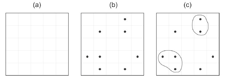
Source: adapted from Stauffer and Aharony, 2018: 1.
Figure 1 Definition of percolation and its clustersNote: (a) shows parts of a square lattice; in (b), some squares are occupied with dots; in (c), the ‘clusters’, groups of neighboring occupied squares, are circled except when the ‘cluster’ consists of a single square.
The percolation process is then applied to the network intersections, represented by interrelated points distributed in a square lattice that have neighboring points within squares that have one side in common (see figure 2 for a schematic illustration of this approach).
Arcaute et al., (2016) also argue that even though a hierarchical structure emerges from the previous network percolation process, it cannot be used by itself to find city limits because morphological properties between cities and regions are different.1 So, to find or have an approximation to those limits at a city level, they appeal to the analysis of the fractal properties of the observed clusters –– in this case, the agglomeration of dots that represents a differentiated urban structure ––, which had proven to be especially useful for identifying thresholds at which city limits are well defined (Arcaute et al., 2016: 2). In finding a maximum of the fractal dimension of the system’s clusters, they uncover a noticeable similarity with other urban data proxies such as satellite images.
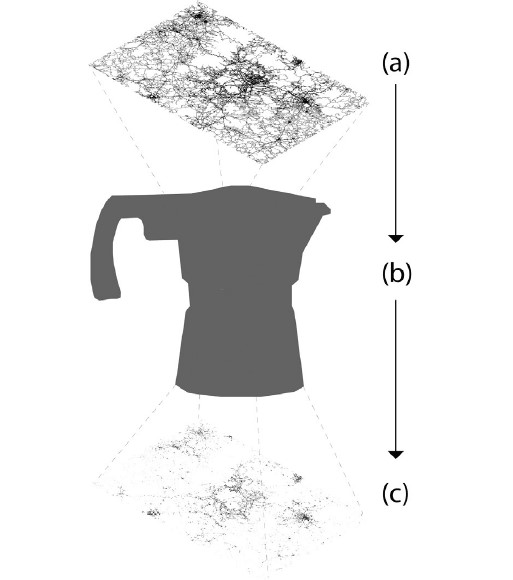
Source: Author’s elaboration.
Figure 2 Percolation process and its clusters in this researchNote: (a) a street network digital data set of an urban system is selected; (b) then, the “size” of a “digital” percolation grid is chosen (i.e., fine, coarse); (c) at the end, depending on the percolating grid size, several clusters at different percolating distances, representing city-like patterns, are obtained as output (data).
2. Fractals and cities
Fractals is a term coined by Benoit Mandelbrot in 1983 for referring to objects:
whose spatial form is nowhere smooth, hence termed ‘irregular’, and whose irregularity repeats itself geometrically across many scales. In short, the irregular ity of form is similar from scale to scale, and the object is said to possess the property of self-similarity or scale-invariance. It is the geometry of such object which is fractal, and any system which can be visualized or analyzed geometrically, whether it be real or a product of our mathematical imagination, can be a fractal if it has those characteristics (Batty and Longley, 1994: 4).
Although Arcaute and colleagues do not make explicit the reason for calculating the fractal dimension in their research (the only explanation given for this is because the fractal dimension has proven to be especially useful in studying the morphology of cities); according to Batty and Longley (1994) and Batty and Xie (1996), we can hypothesize – following other works – that cities are complex systems that can’t be easily measured in an Euclidean way; if cities’ structures rely heavily on physical infrastructure networks (like road and transportation) that resemble fractal-like network geometries because they show self-similarity and scale invariance, and if cities whose fractal dimension grows as the city develops and accommodates more infrastructure become more complex systems2 (West, 2017), then, the fractal dimension is used to measure some sort of complexity degree.3
For Zarza Balluguera, cities are complex systems, and so is their geometry. Since their dynamics are related to non-linearity (see Bettencourt et al., 2007), it could be said their form is an outcome of chaotic processes that, at the same time, can be associated to a fractal geometry (Zarza Balluguera, 1996: 49). For Aguilera Ontiveros, “The emergence of a fractal pattern shows that the spatial structure of an urban settlement […] has an internal arrangement principle, which is characterized by its fractal dimension” (Aguilera Ontiveros, 1999: 54).
Once established cities show fractal-like patterns, it seems obvious to measure the outcome of the percolation process (the resulting clusters) to compare cluster formations at different percolation distances with what we call ‘cities’ using satellite imagery. But again, in Arcaute and colleagues’ work there is no explanation to understand why finding the maximum of the fractal dimension of the urban system shows a high correlation with the CORINE dataset, a land cover series developed by the European Environment Agency.
We already stated that the more developed a city is (i.e., a metropolitan area), the higher its fractal dimension (at least theoretically). Is it possible that the maximum fractal dimension of a given urban system –– which is the one that best correlates with satellite data –– is highly influenced by the moment in which a ‘metropolitan’ cluster is found during the percolation series at different distances? In other words: the maximum fractal dimension could be found when the analyzed urban system reaches the highest degree of complexity.
But a higher degree of complexity of an urban area can be measured in a variety of ways. As mentioned previously, Cao et al., (2020) proposed a novel method inspired in Arcaute et al., (2016) work, by extracting urban areas from multi-source urban data. For them, urban areas are defined as “maximally connected areas that have more urban elements (i.e., population, infrastructure, economic activity) than non-urban areas” (Cao et al., 2020: 241). They percolated ten worldwide urban systems to obtain an optimal urban area threshold using three data sources: population, road network, and nightlights. Then, they validated their results by comparing the derived urban areas from the percolation of those data sources at the maximum value of Shannon’s entropy of each dataset against Landsat imagery, obtaining good agreement with the reference data. In this study, what is remarkably interesting is that they calculated Shannon’s entropy of the size distribution for each cluster system, finding that the entropy reaches a maximum around the critical point, which coincides with the critical point of the fractal dimension. In this regard, we can think further and imagine that city-like patterns could be determined by their complexity of a set of several urban dynamics such as mixed land-use (also using Shannon’s entropy), or the sewer system network, to say the least, represented by the maximum complexity value.
In a very comprehensive study about entropy in urban studies, Cabral et al., (2013) establish the concept of entropy as a contextual-dependent meaning. For instance, it can be a proportion of maximum uncertainty, an optimization of data categories, or the degree of homogeneity or heterogeneity certain cities display in their land use. For them, as cities are systems that resemble complex ones, entropy can be a measure that informs about the fluctuation of the state of the system, ranging from uniformity (lower entropy limit) to chaos (upper entropy limit). In the middle of this index, urban dynamics can show different levels of “organized diversity, redundancy or tolerated disorder” (Cabral et al., 2013: 5231).
Coming back to Cao et al. (2020) findings about this ‘striking’ relationship among critical points of the maximum fractal dimension and the maximum entropy of the very same analyzed urban system, it seems to be an answer for that. While Chen and Huang find both entropy and fractal dimension “can be employed to characterize spatial complex systems such as cities and regions” (Chen and Huang, 2018: 1), Zmeskal et al., (2013: 142) demonstrated that the “entropy of a region of size r can be determined from the radius fractal dimension”, meaning that there is a dependency between those two metrics. Moreover, the fractal dimension can be measured in three ways (for multifractal patterns, like cities): 1) by its capacity dimension (D0); 2) by its information dimension (D1), which “can be seen as Shannon’s entropy” (Arcaute et al., 2016: 7); and 3) by its correlation dimension (D2) (Chen et al., 2017).
When finding a maximum entropy value over their analyzed urban systems, Cao et al. (2020) explain this as follows:
This phenomenon reflects the characteristics of the urban system as an interconnected complex system. Since the intra-city connections are much stronger than the intercity connections, weak intercity connections break up as we increase the threshold [of the percolation]. When the threshold reaches a certain point [the maximum entropy value], all weak inter-city connections do not exist, while the intra-city connections can still be tied closely” (Cao et al., 2020: 5)
This interpretation is in good correspondence with what Chen et al. have found: That “high fractal dimensions suggest low spatial difference and strong spatial correlation between urban parts” (Chen et al., 2017: 599). It could mean that well-defined cities within an urban system show a maximum level of entropy due to higher intra-city connections (compared against intercity connections), and at the same time, a maximum fractal dimension is expressing more cohesion at an intra-city level.
3. Data and Methods
In this paper we studied Mexico’s national road network for 2012 (see figure 3), obtained from the official repository of the National Institute of Statistics and Geography (Inegi, 2012) as is (Step 1). It comprises 4,054,707 edges and 2,699,536 nodes. A first glimpse at the spatial distribution of the road network in figure 3 clearly shows a prominent clustering pattern in the central portion of the country, pockets of empty spaces with lack of connectivity especially in the north and northwest regions of the country, and a collection of inaccessible islands in the northwest.4
In Step 2, we represented the national road network as a graph. It means we split all the network roads into two basic components: nodes (geospatial points representing the intersections between roads) and arcs (geospatial lines representing the roads). This graph is said to be undirected because there is no direction from the edges to the nodes.
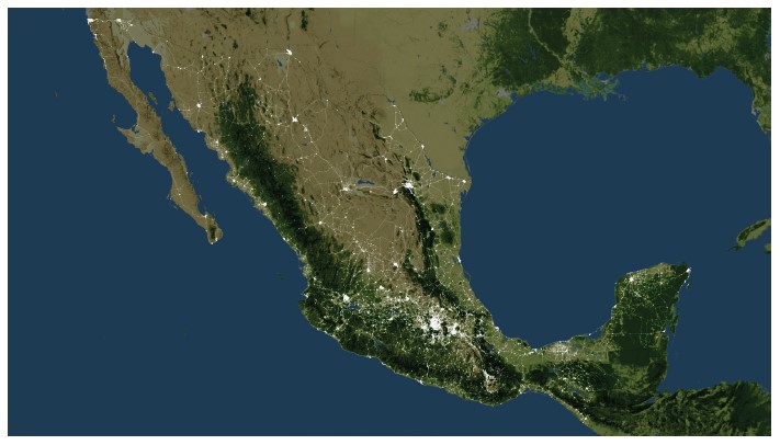
Source: author’s elaboration using QGIS (2020) and data from Inegi (2012).
Figure 3 The spatial distribution of the Mexican road networkNote: a large cluster is visible in the central region of the country with empty spaces in the north and northwest with small inaccessible islands.
After the road network is decomposed into a graph, the percolationprocess begins (Step 3). In this case, when percolating, we filtered geospatialdata recursively with a specific parameter: the threshold distance (d) at which the graph will be filtered (Step 4). The outcome of a single run returns a new graph containing the cluster of reachable nodes using a given distance d (Step 5). Distance d defines what can be traversed from different segments of the network. Lastly, we obtained cluster metrics (Step 6) for each percolated distance. Overall, we repeated the percolation process for different threshold distances, from 100 m to 10 km, every 10 m and, additionally, from 100 m to 190 km, every 100 m, figure 4 shows a schematic diagram of the different steps in the process.
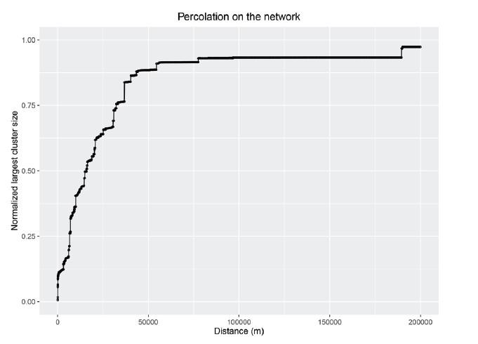
The cumulative cluster size can be plotted to study the behavior of the percolation process. Because it has already been recognized that the road network contains islands, the cumulative cluster size is not expected to reach 1 (see figure 6), as in Cao et al., (2020). That is, there will never be a single cluster containing all the roads even if we percolate up to 190 kilometers. To find the distance at which the percolation outcome contains only one single giant cluster, we should probably use a different road network data source, like OpenStreetMap or an updated and fixed official road network where all nodes are topologically connected.

Following Arcaute et al., (2016), the fractal dimension of the system is calculated at each threshold distance in terms of the scaling relationship between the mass of the clusters and the diameter of their network. The mass is given by the number of nodes . and the diameter is denoted by dmax:
Because we are interested in describing the relationship between mass and diameter, it is useful to express this in logarithmic form:
and study the coefficients of the linear regression of values for all the clusters obtained at a given threshold distance. The slope of this regression gives the value of the fractal dimension for each percolated distance.
Clusters with more than 50 nodes of the percolated road network were considered and plotted on a map. The maximum fractal dimension was obtained by plotting its value as a function of distance. With this new parameter, this subjective cutoff was used in order to take out a great amount of very small and scattered human settlements that characterize the Mexican rural landscape. By doing this, we expect the outcome of the percolated network represents urban settlements more accurately.5
Together with the fractal dimension, we computed Shannon’s entropy, E, for each cluster system:
where N represents the number of clusters in the system, and pi is the proportion of the area of cluster i with respect to all clusters.
Lastly, we performed a two way validation to compare the percolation outcomes at different distances (from 50 m to 1 km) against two different test datasets: the 2014 Global Human Settlement Layer (GHSL) (Florczyk et al., 2019; Schiavina et al., 2019) and Inegi’s 2011 National Land Cover database (Inegi, 2013). Both products use LANDSAT imagery, but the main difference is that the GHSL raster used the built environment layer at a 250x250 m resolution, while the vector Inegi product classifies LANDSAT imagery by land uses and presents them at a 1:250,000 m scale.
In order to make the comparison, we first rasterized the percolated road network nodes at different distances at a unique cell size, raster type and extent, as well as two Inegi’s National Land Cover layers (the human settlements class layer and the urban area one). At this point, all raster files were standardized along with the GHSL, including its projection. It is important to mention that the raw GHSL was cropped to represent only the built environment contained within the SUN 2018 definition. The SUN 2018, National Population Council (Conapo, 2018) is the national classification system of what is ‘urban’ in Mexico. It comprises 74 metropolitan areas, 132 conurbations and 195 urban centers which, overall, add up to 401 cities. Aside from that, a second crop was done: we removed all pixels that had values of built environment below 30%. In this database, each pixel ranged from 0 to 100, depending on the degree of built environment the pixel was able to capture.
Then, the sets of rasterized and percolated road network nodes images were compared against the GHSL, the urban area rasterized layer, and a composed rasterized layer of the human settlements plus the urban area, by two means: a confusion matrix and a similarity index. “A confusion matrix summarizes the classification performance of a classifier with respect to some test data. It is a two-dimensional matrix, indexed in one dimension by the true class of an object and in the other, by the class that the classifier assigns” (Ting, 2010: 209). In this case, the algorithm compares if the values of a given raster match the values of another and it returns two values: The Kappa coefficient and an overall accuracy. “Kappa coefficient, measures the agreement between classification and truth values. A Kappa value of 1 represents perfect agreement, while a value of 0 represents no agreement” (L3Harris Geospatial, 2021: 1).
Since in recent years there seems to be controversy about the suitability of the Kappa coefficient for assessing and comparing the accuracy of thematic maps obtained by image classification6 (Foody, 2020; Sadeghbeygi, et al., 2021), we also applied the Sørensen-Dice index (SDI) for the same validating purpose. Very similar to the Jaccard index, this one (see Dice, 1945; Sørensen, 1948) is used to estimate the magnitude of similarity of two sets of data. It seeks the number of equal elements on both samples and generates a number between 0 and 1, with the latter being a perfect match.
Data processing and algorithms were implemented using the R programing language (R Core Team, 2020). Graphs were constructed using the igraph package and were processed using a parallel approach with 24 cores and 126 GB of RAM. Code is available at http://gitlab.geoint.mx/tapiamcclung/percolation
4. Results
The first and most relevant discovery in this research is that, as in Arcaute et al., (2016) and in Cao et al., (2020), the Mexican urban system percolated through its road network (nodes) behaved as expected: it shows a maximum fractal dimension at 250 m and a maximum Shannon’s entropy at the very same distance (see figure 5). Even though our maximum critical points of both fractal dimension and entropy are close to those previous researches (300 m), as stated in Arcaute et al. (2016), the distance at which the maximum fractal dimension emerges (the critical point) should vary among different geographies because it depends on the spatial arrangement of the road network in relationship with its topography. This confirmation is relevant because these critical points seem to very accurately define the limits of what we call ‘cities’.
Figure 6 shows a plot of the cumulative cluster size and the percolation distance. It can be seen that beyond 50,000 m there is very slow progress on the formation of one big cluster (all the Mexican roads network towards becoming just one cluster, with the exception of islands mentioned before). But what is more relevant to percolation theory, is when the system reaches a critical point. In this case, when both entropy and fractal dimension reach their maximum. As we can see in figure 7, the percolated network at 250 m seems to accurately delineate the national urban system.
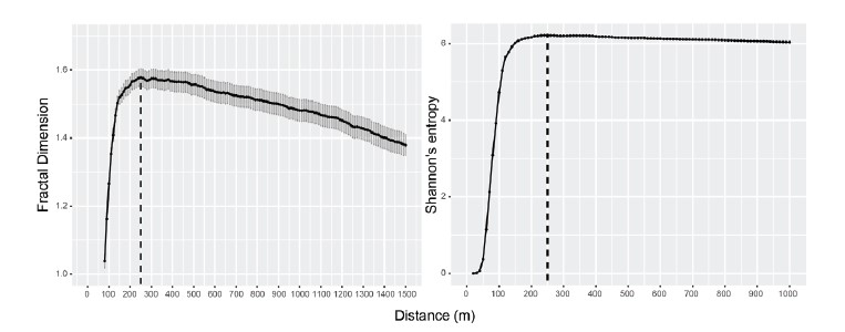
Source: author’s elaboration using R (R Core Team, 2020).
Figure 5 Fractal dimension and Shannon’s entropyNote: a) shows the fractal dimension of the percolation on the network for clusters with more than 50 nodes; b) shows Shannon’s entropy values. Note that both, fractal dimension and entropy, reach a critical point (maximum value) at a threshold distance of 250 m.
Source: author’s elaboration using R (R Core Team, 2020).
Figure 6 Cumulative normalized largest cluster size as a function of threshold distance
Source: author’s elaboration using QGIS (2020) and data from Inegi (2012).
Figure 7 Map showing the Mexican road network percolated at 250 mNote: clusters formed after the percolation process largely correspond to what we describe as cities within the National Urban System. Clusters with less than 50 nodes are excluded
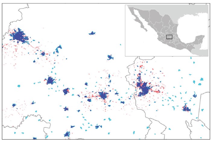
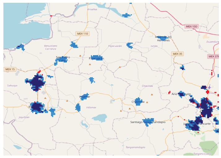
Figure 8 presents a portion of the central part of Mexico in which the percolated nodes at 250 m (light blue) are superimposed with the GHSL 2014 (red). The intersection between those two sets is depicted in dark blue. This representation clearly shows that percolated nodes at 250 m (where both the maximum fractal dimension and entropy are found) are in very good correspondence with what Cao et al., (2020) and explain when they find their optimum threshold (their maximum entropy): that when this maximum is reached, higher intra-city relationships within all the analyzed clusters in a given urban system are made explicit. After reaching this threshold, the maximum fractal dimension and entropy will steadily decrease (see figure 5), probably because the remaining percolated nodes at larger distances will only add weaker inter-city connections to the maximum reached complexity. As can be seen in figure 8, most of the red pixels are arranged along highways or secondary roads that connect cities or towns, and accordingly, they do not form part of the city itself. We could therefore say they are part of the ‘rural’ domain. Also, those isolated clusters in light blue are very small human settlements (ranches, rural towns) and most of them do not exceed 5000 inhabitants. The fact that the percolation process returns clusters of this type is not an error by itself. Rather, it is an opportunity to rethink what is urban and what is not, since the method clearly shows the existence of small human settlements that are on track to becoming urban, given their installed infrastructure. Figure 9 shows a closer look of this particular region. Those small urban settlements are well recognized by this method, although hardly recognized by satellite images.
Source: author’s elaboration using QGIS (2020) and data from Inegi (2012) and GHSL (Florczyk et al., 2019).
Figure 8 Results for the central part of MexicoNote: percolated nodes (2012) at 250 m are shown in light blue, GHSL (2014) in red and the intersection of the percolated nodes at 250 m and the GHSL in dark blue.
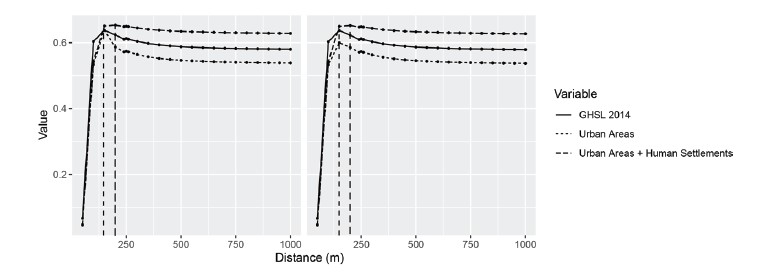
Another relevant finding is that our percolated Mexican urban system is in very good correspondence with what is officially recognized as urban (see also figure 7). Figure 10 and Table 1 show the outcomes corresponding to the comparison between the percolated nodes of the national road network at different distances against the GHSL 2014 and Inegi’s National Land Cover database for 2011 for both the Urban Areas layer and Urban Areas + Human Settlement layer by calculating the Kappa coefficient and the Sørensen-Dice index (SDI). The best correlation reaches a fair correspondence (over 65%) at 200 m, which is very close to the optimal entropy and fractal dimension thresholds of 250 m.
Source: author’s elaboration using QGIS (2020) and data from Inegi (2012) and GHSL (Florczyk et al., 2019).
Figure 9 Detail of the results for the central part of MexicoNote: percolated nodes (2012) at 250 m are shown in light blue, GHSL (2014) in red and the intersection of the percolated nodes at 250 m and the GHSL in dark blue. Many known rural towns (light blue) are well recognized by the percolation process but not by satellite images (red).
Source: author’s elaboration using R (R Core Team, 2020) and data from GHSL (Florczyk et al., 2019) and Inegi (2012, 2013).
Figure 10 Comparison of the Sørensen-Dice index and the Kappa coefficientNote: we compare the percolated national road network with more than 50 nodes versus GHSL 2014, Urban Areas and Urban Areas +Human Settlements Layers, dashed vertical lines indicates the distance at maximum similarity/accuracy (Inegi’s National Land Cover database).
Table 1 Comparison of the Sørensen-Dice index and the Kappa coefficient values
| Sørensen-Dice index | Kappa coefficient | |||||
|---|---|---|---|---|---|---|
| Distance (m) | GHSL 2014 | Urban Areas | Urban Areas + Human Settlements | GHSL 2014 | Urban Areas | Urban Areas + Human Settlements |
| 50 | 0.06692467 | 0.04842445 | 0.045313435 | 0.066779 | 0.048276 | 0.045162 |
| 100 | 0.6038661 | 0.53371208 | 0.543541973 | 0.603161 | 0.532898 | 0.542588 |
| 150 | 0.63808538 | 0.63808538 | 0.651013584 | 0.637251 | 0.600051 | 0.650016 |
| 200 | 0.62379382 | 0.58694193 | 0.653771038 | 0.622874 | 0.585958 | 0.652706 |
| 240 | 0.61091195 | 0.57203306 | 0.649127422 | 0.60993 | 0.570983 | 0.648005 |
| 250 | 0.61305186 | 0.5741182 | 0.649993079 | 0.612079 | 0.573077 | 0.648879 |
| 260 | 0.61091195 | 0.57203306 | 0.649127422 | 0.60993 | 0.570983 | 0.648005 |
| 300 | 0.60424055 | 0.56427088 | 0.645140839 | 0.60323 | 0.563189 | 0.643989 |
| 350 | 0.59787419 | 0.55704373 | 0.640825075 | 0.596837 | 0.555933 | 0.639644 |
| 400 | 0.59353954 | 0.55225878 | 0.638259935 | 0.592484 | 0.551129 | 0.63706 |
| 450 | 0.5904219 | 0.54905699 | 0.636128545 | 0.589354 | 0.547914 | 0.634915 |
| 500 | 0.58797856 | 0.54670994 | 0.634566835 | 0.586901 | 0.545558 | 0.633344 |
| 550 | 0.58644481 | 0.54486411 | 0.633422538 | 0.585361 | 0.543705 | 0.632192 |
| 600 | 0.58516479 | 0.54345816 | 0.632570509 | 0.584076 | 0.542294 | 0.631334 |
| 650 | 0.58397139 | 0.54214335 | 0.631616086 | 0.582877 | 0.540974 | 0.630374 |
| 700 | 0.58311675 | 0.54124088 | 0.631012873 | 0.582019 | 0.540068 | 0.629768 |
| 750 | 0.58251297 | 0.54055089 | 0.63045827 | 0.581413 | 0.539375 | 0.62921 |
| 800 | 0.58204858 | 0.5399837 | 0.630016862 | 0.580947 | 0.538806 | 0.628766 |
| 850 | 0.58161549 | 0.53947904 | 0.629607812 | 0.580512 | 0.538299 | 0.628355 |
| 900 | 0.58109588 | 0.53894923 | 0.629133436 | 0.579991 | 0.537768 | 0.627878 |
| 950 | 0.58072603 | 0.53860162 | 0.628858711 | 0.579619 | 0.537419 | 0.627602 |
| 1000 | 0.58045684 | 0.53827843 | 0.628655794 | 0.579349 | 0.537094 | 0.627398 |
Note:we compare the percolated national road network with more than 50 nodes versus GHSL 2014, Urban Areas and Urban Areas +Human Settlements Layers, dashed vertical lines indicates the distance at maximum similarity/accuracy (Inegi’s National Land Cover database). Maximum values are highlighted.
Source: author’s elaboration using R (R Core Team, 2020) and SAGA (Conrad et al., 2015) with data from GHSL (Florczyk et al., 2019) and Inegi (2012, 2013).
There could be several reasons as to why the maximum values of these indices are not reached at exactly the same distance as the maximum fractal dimension and entropy. Since 1970 there have been several attempts to delimit metropolitan areas in Mexico. In 2004, the Ministry of Social Development (Sedesol), the Conapo and the National Institute of Statistics and Geography (Inegi) defined the criteria by which municipalities would become part of a metropolitan area, including physical conurbation, functional integration, and urban character (Anzaldo, 2019). Aside from these traditional criteria, they included two other considerations which seem to distort the former geospatial considerations: one is due to political considerations; the other due to planning considerations. Whether it clarifies or not what that implies, Anzaldo states that:
They are municipalities that, due to their particular characteristics, are relevant and are recognized by the federal and local governments as part of the metropolitan areas, through a series of instruments that regulate their urban development and the planning of their territory (Anzaldo, 2019: 36).
Those rules are still valid in the latter metropolitan area delimitations (Conapo, 2012, 2018), and are implicit within our test databases, so the ‘lower’ Kappa and SDI similarity index could be understood as cumulative errors not imputable directly to our geospatial process, but to a definition of what is urban or not in the national urban system, and due to errors among the used datasets. In this regard, we could say that Arcaute and colleagues’ validation method is pretty similar to ours.
Several types of errors are inherent to the used databases. Others can be imputed to the method itself. Relating the latter, we observed that some intra-city areas were not included within the urban clusters because of their block size (i.e., intra-urban industrial areas, or train facilities that had blocks larger than 200 m). Another issue is related to the subjective cut off for mapping clusters with more than 50 nodes. In doing this, several rural towns (even parts of cities) could be ‘lost or found’ depending on this subjective threshold.
Regarding errors inherent to the used databases, for instance, satellites used for developing the GHSL do not clearly recognize all the built-up environments in desert areas or within very large green areas at the 250 x 250 m resolution. In the Inegi Land Cover Layer, we found large industrial areas, exurban gated communities and other types of large facilities classified as urban (i.e., oil refineries, airports, golf courses, etc.). And in Inegi’s National Road Network layer there are a lot of redundant or missing vertices along the arcs (topological errors). Also, the year disparity between databases or simply having an outdated database lead to mistaken validating readings. Nevertheless, the outcomes are very promising to continue seeking alternative ways to define what is urban and what is not, in a more automated and less subjective manner.
Conclusions
Despite establishing the relationship between the maximum values of both the fractal dimension and Shannon’s entropy, some questions still lack clear answers: Why is it that at this ‘critical point’ is where the percolated national road system resembles more what is officially recognized as urban? Could it be possible to use this methodology to precisely discriminate between what is urban and what is not? Why is 200-300 m a percolation distance that seems to differentiate urban regions from others that do not seem to fit in the same category?
There seems to be a reasonable explanation for this. Road network infrastructure is one of the most distinctive characteristics of urban life. Moreover, its density or agglomeration within a specific territory (as demonstrated by Cao et al., 2020) shapes a lot of human settlement dynamics, such as commuting, land-use and travel behavior, among others. It defines the way people move around geography. The more complex the local road network is, the more intricate urban dynamics we can find. But what remains unclear is how the fractal dimension and Shannon’s entropy capture this complexity, even understanding the rationale of the equations. Translating this into public policy for defining what is urban and what is not, is not a trivial task. More tests and research are needed in order to better explain this apparent relationship.
Regarding the 200-300 m range of the percolation distance as a good proxy for defining what is urban, it probably has more to do with local ways for planning the city or the organic growth of the city itself. It is known that most people in cities tend to walk no more than 500 m to reach transit infrastructure, and that most Mexican cities have blocks of less than 100 m in length. However, there are a lot of larger urban blocks so this method should be refined to take into account this variation of dimensions. As stated before, several parts of cities may have not been properly captured due to this. Also, this range varies among cities circumscribed within a national system, so we think this methodology cannot be applied globally, as in Cao et al., (2020), as several local characteristics are at play (e.g., topography). In this sense, that range would surely vary according to local urbanization and metropolization traditions.
One of the key issues related to the subjectivity of this methodology relies on the percolated road network nodes threshold that are removed when calculating the fractal dimension and Shannon’s entropy. Those removed clusters (in this case, when there are less than 50 nodes conforming a cluster) should be very carefully evaluated. As explained before, a lot of them represent very small and scattered human settlements. In future research, it is mandatory to establish a relationship between the minimum population that defines a town and the minimum number of nodes that form a cluster. By doing this, validation against satellite images could be substantially improved. Derived from previous research, we already know there is a quasi-linear relationship between city size and population, so this should not be problematic.
Our research presented a method that depends on the availability of a road network dataset. In this case, we percolated the network using the arcs. But as stated before, there are several ways to calculate the fractal dimension using the same dataset (it could be done by different methods, i.e., box-counting, radius, nodes, arcs) and for different databases (buildings, built-up area, roads, land-use). We should explore the idea that other constituting elements of what urban life is can be measured in order to widen the vectors of elements that add to the definition of what is urban.
Clearly, this method could also help determine urban sprawl to some extent (different methodologies and different data sources combined), but it could probably be useful for detecting clusters of other types of social dynamics, such as agglomeration economies and diseconomies, the degree of mix-land use, or even contribute to different kind of regionalization for criminal behavior, for example.

