


 nueva página del texto (beta)
 Inglés (pdf)
 Artículo en XML
 Referencias del artículo
 Enviar artículo por email
 Citado por SciELO
  Similares en
SciELO
Similares en
SciELO 
 Permalink
Introduction
In recent years, many studies have focused on solving the problem of chatter-free mechanisms. On the other hand, new proposals have been made to obtain control algorithms capable of developing bell-shaped speed profiles whose task is to emulate the speed profiles described by human limbs. Tasks such as the transport of dangerous substances or liquids that can spill show the importance of eradicating inertial effects, achieving a bell-shaped speed profile.
For example, the way a human being generally moves his hand along a more or less straight path from one point to another shows common invariant kinematic features such as a bell-shaped speed profile (Morasso, 1981), many models have also been proposed; for example, "a minimal torque-change model" (Uno et al., 1989), "a minimum jerk model" (Flash & Hogan, 1985), both models can generate hand trajectories in good agreement with the experimental data. Furthermore, in Yeung & Chen (1988) a variable structure model following control design (VSMFC) for robotic applications was presented in which the chattering problem was solved. In Chen et al. (1990) a control algorithm was proposed where the inverse of the inertial matrix was not required. Another method that uses an electrostatic potential field and a sliding mode for a manipulator that regulates the movement time but not the dynamic behavior of a robot has been presented in Hashimoto (1993). In addition, Morasso (1993) proposed a Time Base Generator (TBG) that generates a time series with a bell-shaped velocity profile, and showed that the trajectory of a hand can be generated with a transnational speed and rotational speed with a TBG signal.
On the other hand, Sira (1992) and Zhang & Panda (1999) have proposed an involved dynamic sliding mode control technique for a general class of nonlinear systems. However, the strict requirement of the measurement of the slip surface derivative is necessary, so Tsuji et al. (1995) proposed a method with a TBG in artificial potential field approach (APFA) that can regulate the time of motion and also the speed profile of the robot but it cannot be applied to dynamic control. In 1998, a new method is developed introducing the combination of a time scale transformation with a TBG, the method is useful for robot time scheduling problems (Tanaka et al., 1998). In addition, a new stability analysis and design procedure for variable structure robotic controllers with PID-type sliding surfaces was presented, the controller is simple and robust (Stepanenco et al., 1998).
A human-like trajectory is generated for the robots with the TBG-based trajectory generation method (Tanaka et al., 1999), then the TBG generates a target spatial and temporal trajectory for the robot (Tanaka et al., 2000). A novel chattering-free dynamic slip mode controller is proposed for a time-varying sliding regime for all times and for any initial conditions (Parra, 2001). Subsequently, a Cartesian control system is proposed in (Dominguez et al., 2008), which guarantees a robust tracking in finite time based on a time base generator for uncertain robotic arms, to achieve this goal we proposed a nonlinear control based on modes second-order sliders, however this method only works on robots without gravity. Another alternative to reduce the inertial effects has been presented in (Kuo et al., 2011). The chatter effect is addressed in García et al. (2011). On the other hand, a non-chattering sliding mode controller is proposed, the new sliding surface is parameterized by a base time generator (Gashemi & Nersesov, 2013). Chatter is a phenomenon that has been sought to eliminate through many methodologies, thus a new sliding mode controller with a continuous control strategy has been proposed to achieve a chattering-free controller (Feng et al., 2014). A new controller with faster response and gravity compensation was introduced in Huang et al. (2014), Nonlinear Proportional Derivative (NPD) controller has smaller errors than conventional Proportional Derivative (PD) controllers.
In this paper we present a robust control algorithm for one degree of freedom mechanisms that solves the problem of inertial effects, eliminates chattering and presents a bell-shaped speed profile. The algorithm is based on a sliding mode control and a time base generator, the algorithm reaches a desired position in a finite time, the algorithm is adaptable to any mechanism of one degree of freedom and is applicable to tasks that require precision, the future scope of this research is to apply the algorithm to robotic arms, such as prostheses or mechanisms focused on rehabilitation, future studies to mechanisms of two or more degrees of freedom.
Modelling
Kinematic model-vector loop method
This section presents the kinematic and dynamic analysis of a one degree of freedom mechanism. The mechanism has a rotary actuator that generates the displacement q in the point, and point C is vertically displaced.
Figure 1 shows the kinematic constraint equation. R1, R2 and R3 are the vectors that describe the loop equation (1).

The angles are defined with respect to the positive X-axis and the vectors are defined by equations (2), (3) and (4).
For position analysis we define the vector P as the unknown variables that determine the position.
With the components of each position vector, the kinematic constraint functions (6) and (7) are obtained, the functions are equal to zero because the geometry of the mechanism is closed.
With the kinematic constraints, the position matrix (8) is found, now it is possible to know the position of the mechanism at any time:
The kinetic energy of the mechanism is obtained from the velocity analysis, therefore F is the matrix of the kinematic constraint functions of the mechanism:
Differentiating the matrix of the kinematic constraint functions with respect to time, the velocity is obtained:
From (10) the acceleration is derived:
The matrices are solved using Wolfram Mathematica®.
Mechanism dynamics
The dynamic model of the mechanism used in this paper can be written as follows:
Where
Therefore, substituting (13) and (14) in (12), the dynamic model components are rewritten as:
Jacobian Extended:
Inertia Matrix:
Matrix of centripetal and Coriolis forces:
Gravitational vector:
The dynamic model is solved with Wolfram Mathematica® and the solution is validated using: Working Model® vs Matlab-Simulink®. Figure 2 shows the validation of the dynamic model in terms of the generalized variable q. The simulation conditions are shown in Table 1.

Figure 2 Dynamic model validation: a) “q” position
Table 1 Validation parameters of the dynamic model in the Matlab-Simulink® software
| Simulation parameters. | Value |
|---|---|
| Tau (𝑈) | 0.001 Nm |
| Solver | Ode4 (Runge-Kutta) |
| Sampling time of simulation | 3 s |
| Integration step | 0.001 |
Figure 3a shows the position of the generalized variable q, the velocity of the generalized variable is shown in 3b and finally 3c shows the acceleration. The graphs in magenta color correspond to Matlab-Simulink®, while the graphs in black color correspond to the Working Model®. For all three cases the graphs converge.

Control algorithm
The algorithm presented in this paper is a robust technique for nonlinear systems that operate under conditions of uncertainty. The sliding mode control reduces the sensitivity to the variation of uncertainties and external disturbances.
Time base generator
The time base generator equation (22) is written as a time function (21), where
In addition, equation (21); being a non-forced time-varying function allows the time base generator to be analyzed like error function, being possible to combine it with the sliding mode control law.
Where:
In equation (22),
Where
In Tanaka et al. (1998) a new trajectory generation method for an omnidirectional mobile robot has been proposed, equation (24) has been used to generate a composite time scale, where the convergence times are defined according with
The system converges to the equilibrium point in
From (22),
The time base generator must be defined by the designer of the controller, such that
The trajectory
Therefore, equation (27), (28) and (29) show that the desired trajectory is fulfilled.
Where the parameters assigned to demonstrate the trajectory are:
Now equations (27), (28) and (29) becomes the system (30).
Then the system is solved, obtaining as a result:
The results are shown in Figure 3, the convergence time is 5 seconds.
Figure 3 shows that the trajectories established in (21) and (22) are true, and this allows the mechanism to be taken from one point to another in a finite time. On the other hand, the α gain is responsible for bringing the error to zero in transient space in a finite time.
Sliding mode control
The position control is proposed in the joint space; where q is the position and qd is the target position (Figure 1). Therefore, the errors are:
In this paper we introduce the TBG as a function of time (21) to the slip surface (33) with the intention of trapping the system in the stable state and not allowing disturbances, making the error smaller each time. Therefore, the sliding surface proposed for the control law is.
Substituting errors of position (31) and speed (32) in sliding surface (33), the new sliding surface can be written as:
In Parra (2003) the sgn function is used to catch the error in the sliding surface, then the next equations have been proposed:
Where
In the equation (36), t represents the final time, t0 the initial time, k is a positive constant, S is the sliding surface and
Therefore, the sliding mode control law can be written as:
The control law that is applied is by sliding modes. The sgn function allows catch the error on the sliding surface, however, the tanh function a smoother displacement is obtained, which helps to reduce chattering in the motor.
Therefore, the equation (38) is the control law, however to achieve more robust control a PID is applied. The PID is defined in a general way in (39).
Where
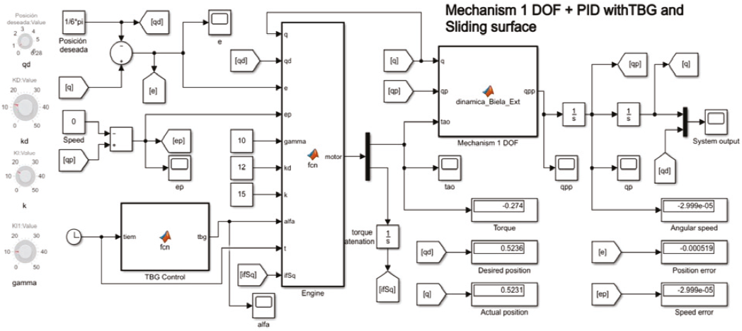
Figure 4 shows the block diagram of the control algorithm. The control law (40) was programmed in Matlab-Simulink®, Figure 5 shows the feedback of the instantaneous position, in left is the function corresponding to the TBG, also the dynamic model is showed. The block "engine" has the control law.

Results
This section shows the results obtained by two joint position control tests. The tests consist of bringing the mechanism from one position to a desired position in a given time.
The time base generator applies the control law to synchronize the mechanism at the desired convergence time. The TBG only adjusts the α gain in the control algorithm based on operator-specified time and does so in a transient space. The sliding surface makes the error converge more smoothly towards 0, the sliding surface has action in the transient space.
The simulations have been carried out in the Matlab-Simulink® software, using the model in Figure 5.
Test 1
The initial position of the mechanism is 0 rad and the objective is to move the mechanism to the desired position of π/2, in a finite time of 3 seconds. The α gain is adjusted based on the desired convergence time. Therefore, for this test the α gain has a constant value.
Table 2 shows the initial position, the desired position and the simulation conditions. On the other hand, Table 3 shows the tuning gains in the controller and finally the graphical results are shown below.
Table 2 Simulation data for joint control in Matlab-Simulink. Test 1
| Simulation parameters | Value |
|---|---|
| Desired position (qd) | π/2 |
| Initial position (q) | 0 rad |
| Solver | Ode4 (Runge-Kutta) |
| Convergence time (TBG) | 3 s |
| Integration step | 0.001 |
Table 3 Gains in the controller for joint position control in Matlab-Simulink. Test 1
| Gains in the controller | Value |
|---|---|
| Gain α in TBG | 10.7 |
| Gain k | 15 |
| Gain kd | 12 |
| Gain ki | 0.001 kd |
| Gain kp | (kd)(α) |
Figure 6 shows the evolution of the movement described by the mechanism, in the upper part the magenta line indicates the desired position, while the black line describes the change in position of the mechanism. Near second 3 a convergence between both lines is observed. Three seconds was chosen as time of arrival at the desired position and based on this the alpha gain was calculated.

Figure 6 also shows that the arrival at the desired position does not present oscillations, as shown in some conventional PID controllers. This shows that vibrations and inertial effects are eradicated with the algorithm proposed in this article.
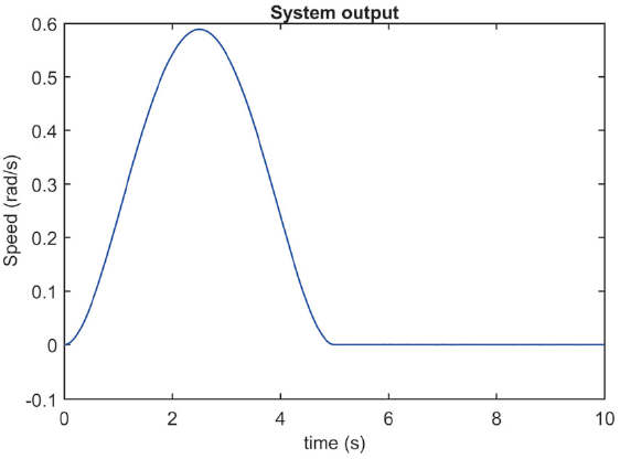
Figure 7 shows the speed profile of the movement performed by the mechanism to reach the desired position in the proposed time. A bell-shaped speed profile has been showed, starting at time (t=0) and gradually increasing until it reaches a maximum value at half the total movement time, at which point the speed gradually decreases until it reaches zero again.

The speed profile obtained shows that there is no over-acceleration at the beginning of the movement, thus demonstrating that the inertial effects have been canceled by the action of the control algorithm. On the other hand, the speed profile shows that the movement described by the mechanism is a smooth and precise one. During the travel time, no disturbances are observed in the speed curve, therefore, the external disturbances are also canceled by the control algorithm.
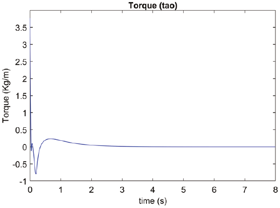
Figure 8 corresponds to the behavior of tau in the motor, it can be seen how tau does not present chatter, which again shows that the inertial effects have been canceled by the control algorithm.
The Table 4 shows the results obtained in test.
Test 2
Test 2 is similar to test 1 with a change in some parameters to verify the functionality of the control algorithm.
Table 5 shows the initial position, the desired position and the simulation conditions, Table 6 shows the tuning gains in the controller and finally the graphical results are shown below.
Table 5 Simulation data for joint control in Matlab-Simulink. Test 2
| Simulation parameters | Value |
|---|---|
| Desired position (qd) | π |
| Initial position (q) | π/2 |
| Solver | O de 4 (Runge-Kutta) |
| Convergence time (TBG) | 5 s |
| Integration step | 0.001 |
Table 6 Gains in the controller for joint position control in Matlab-Simulink. Test 2
| Gains in the controller | Value |
|---|---|
| Gain 𝛼 in TBG | 6.4 |
| Gain k | 15 |
| Gain kd | 12 |
| Gain ki | 0.001 kd |
| Gain kp | (kd)(α) |
As in test 1, the result of the position graph is satisfactory. The mechanism reaches the desired position in the stipulated time. There are no oscillations in the movement, indicating that the inertial effects have been canceled (Figure 9).

The speed profile observed in Figure 10 is in agreement with what was expected. A bell-shaped velocity profile has been shown, it starts at instant zero and ends at second number 5 in accordance with the time stipulated in TBG. Let us remember that α gain is adapted according to the desired convergence time. The speed profile shows no vibrations or over acceleration.
Finally, Figure 11 shows the behavior of the tau, in the graph chattering is not observed. Table 7 shows the Test 1 results.

Conclusions
A robust control algorithm is introduced to cancel the inertial effects and achieve a chatter-free control, the algorithm has a sliding surface to ensure smooth convergence of error to zero, and a hyperbolic trigonometric function has been applied to decrease chattering. A time base generator (TBG) has been applied to reach a desired position in a finite time, in addition to obtaining a bell-shaped speed profile that ensures that over-acceleration and oscillations are eliminated when reaching the desired position. Also, a PID controller is added to make the algorithm more robust. The algorithm can be adapted to any one degree of freedom mechanism. The bell-shaped speed profile suggests that it can be applied to robots that aim to simulate the behavior of human limbs and to future research in the field of physical rehabilitation.

