Purpose of this work

Numerical fluid flow modeling is a challenge that has seen numerous approximations, most of which are focused on a set of phenomena for a particular application or certain boundary conditions. At the time, there is no general approach, analytical or computational, that provides physically accurate results consistent with experimental observations; such is the stochastic nature of fluid dynamics, even in cases with very simple boundaries and invariant physical properties. Recent publications continue to tackle this problem applying time-proven techniques such as the combination of numerical and physical experiments such as the case studied by (^{Zambrano et al., 2017}) or the synthesis of correlations for a very particular flow configuration, as is the case of (^{Jiménez et al., 2020}). Another common approach is the application of pre-calibrated CFD models (^{Klapp et al., 2020}) or the study of analytical solutions for academic purposes as outlined by (^{Cozzolino et al., 2015}). During the 2000s and 2010s, most computational fluid dynamics (CFD) applications both in academic and professional contexts, are known to be based on finite volume methods (FVM) and finite element methods (FEM) (^{Blazek, 2015}). Well-known commercial software packages such as Fluent, which is based on FVM, provide a stable platform for problem setup, solving and postprocessing stages, making the method widely available for professional and research purposes.

Much less frequent applications are found in studies that use mesh-free methods such as smoothed particle hydrodynamics (SPH) and other alternatives (^{Dutra, 2018}; ^{Pozrikidis, 2016}). The SPH method was originally formulated in 1977 for problems on stellar mechanics (^{Gingold & Monaghan, 1977}). The modifications and variants that are required to adapt this method to the general case of fluid mechanics were developed in the 1990s (^{Monaghan, 1992}), mainly for the correct modeling of the interaction with solid boundaries and adapting better neighboring particle search algorithms, a key factor in ensuring that the computational cost is at an advantage in comparison to other CFD methods.

Between 2010 and 2020, a considerable number of scientific articles have been published on the subject of SPH in relation to the mathematical formulation (^{Antuono et al., 2010}; ^{Hu & Adams, 2015}; ^{Jin et al., 2015}), the experimental calibration of variants of the method for particular applications (^{Cao et al., 2014}; ^{Deng et al., 2013}; ^{Fourtakas & Rogers, 2016}), and the hybridization with other methods for the modelling of elastic and elastoplastic solids modeling (^{Duan et al., 2017}; ^{Hu et al., 2015}; ^{Mardalizad et al., 2017}) or viscoplastic flow (^{Brezzi et al., 2017}; ^{Han et al., 2019}; ^{Heck et al., 2017}). Also in this period, monographs on the subject (^{Liu & Liu, 2003}; ²⁰¹⁵), (^{Violeau, 2012}) have been published and highly optimized open-source code libraries such as SPHysics (^{Cabrera et al., 2015}) have become available. However, SPH is far from being accepted as an industry standard or being routinely incorporated in commercial software for engineering problems, but it does have advantages where low-cost parallel processing platforms based on current GPU architecture can be taken advantage of so that processing times can be significantly reduced.

The purpose of this article is to introduce the reader to the main concept of the SPH method and to show some of the practical aspects of its implementation, use and expected accuracy through the application to two well-known hydraulics problems. Although other authors have studied similar applications of SPH in order to calibrate the numerical model, the boundary conditions and associated experimental data referred to in this article have not previously been used for verification of models by SPH. Furthermore, the results of this process provide direction for future work in the development of complements applicable to the SPH method in particular and potentially to CFD in general.

An outline of the SPH method

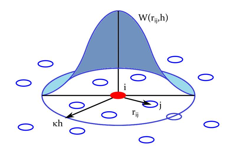
The smoothed particle hydrodynamics (SPH) method is a discrete meshless technique in which the fluid volume is divided into a finite number of particles whose position is not fixed (Lagrangian approach), unlike meshed methods in which the nodes do not change position (Eulerian approach). The movement of these discrete particles is driven by the fluid dynamics equations and physical state equations, such as those that drive changes in density, viscosity or energy state. Unlike other particle methods, in SPH, not only the interactions of a particle with immediately adjacent neighbors are considered, but also those within a zone of an arbitrary radius of κ h as shown in Figure 1. Here, h is a numerical parameter known as the smoothing length and is usually chosen between 1.1 and 1.7 times the average particle size; κ is an empirical constant that is usually fixed at 1.1 (^{Liu & Liu, 2003}). So that the interactions are not artificially distorted, the farther away the neighboring particle is, the less it affects its neighbor, an effect made possible by the use of a weighting function called the smoothing function W(r _ij , h) , that is specially defined for this purpose (^{Monaghan, 1992}). This smoothing function is dependent on an absolute interparticle distance magnitude r _ij and the smoothing length h .

Figure 1 Visual representation of smoothing function W(r _ij , h)  

If the size of this area is correctly chosen (through a proper value of h and the adjustment of κ), the process of obtaining a weighted local value of the physical variables of interest helps stabilize the calculation, since it is a volume integral that smooths numerical variations within it. This approach is known as the kernel approximation (^{Liu & Liu, 2003}), and is subsequently approximated numerically using additional, more conventional methods for the integral and derivatives of the variables of interest. This step is known as the particle approximation (^{Liu & Liu, 2003}).

This process, whose mathematical foundation can be seen developed in vector notation in the monographs cited previously, make it possible to calculate the value f(x) of any variable of interest pertaining to a particle i surrounded by N neighbors that make up part of the flow. The position of the particle x _i must be known (making this scheme an explicit forward time-step method) so that f(x _i ) can be obtained with Eq. (1), which can be transformed relatively directly to computational source code for use in applications.

In this equation, W(r _ij , h) is the function that fulfills the weighting effect of variables, and since it decreases to zero as the absolute value of r _ij increases (the distance between particle i and a neighboring particle j ) it produces a numerical smoothing effect in a manner similar to a weighted average. Parameters h and κ, as mentioned before, are chosen according to the type of flow and mean expected flow speeds, to determine how many of the nearby particles will be considered within the weighting. The selection of the smoothing function itself depends both on the mathematical properties it must have as to not alter the physical phenomena being modeled, and on the influence it may have on numerical stability (^{Monaghan, 1989}; ^{Agertz et al., 2007}).

Since the equations of fluid dynamics and their physical state equations require some of their derivatives, it can be shown (^{Liu & Liu, 2015}) that the divergence of f(x) evaluated for a particle i with a known position x _i can be approximated by Eq. (2).

Since the kernel function itself W(x,h) does not change, the value of the gradient ∇ W(x,h) can be obtained analytically, thus arriving at Eq. (3) for use wherever derivatives are required.

The density term in Eq. (1), not only affects the value of f(x) but also drives its stable variation, to such an extent that if an incompressible fluid is to be modeled, one approach to avoid numerical instabilities is to add an artificial compressibility (^{Zhang & Hu, 2017}). The addition of such an equation of state for nearly incompressible fluids is generally known as the weakly compressible SPH (WSPH) method, and it is a common approach to avoid unnatural, apparently random movements of particles due to inelastic interaction with solid boundaries, among other phenomena. This is especially true when particle velocities are low (^{Rossi et al., 2017}).

The previous outline describes the general concept of SPH as a numerical method applicable to solving the equations of fluid dynamics as shown by the considerable number of publications that mention the use of SPH applied to numerical modeling. Recently, novel implementations of SPH have focused on its hybridization with FVM and FEM, as well as on the precise modeling of boundary phenomena and non-linear behavior of fluids. A good starting point for a review of the first serious growth of SPH as an applied method that occurred between 2000 and 2010 is in (^{Monaghan, 2012}). An up-to-date comprehensive assessment of the state of the art and remaining challenges for the method can be found in (^{Vacondio et al., 2020}).

Implementation and original source code

It is clear that the basic implementation of the SPH method has been well studied and its applications evolved both from a computational and an experimental point of view. Many cases have been solved and the results compared with measurements on physical experiments about phenomena of general interest such as the discharge of a jet in stationary medium (^{Espa et al., 2008}), flow in a channel (^{Federico et al., 2012}), or dam break (^{Shao & Lo, 2003}), among many others with a much more specific purpose, such as the few reference examples mentioned in the introduction. A proper review of industrial applications can be found in (^{Shadloo et al., 2016}).

However, since part of the research objective was to assess the practical implications of modifying the method from its foundation, prior to the implementation of common correction algorithms, a totally original implementation of the numerical method was written in C programming language. No programming libraries were used, which resulted in first-hand contact with all the computational stages involved in a WSPH model. The first version of the functional source code, named Gap-SPH, is a three-dimensional implementation of the classic SPH formulation for linear fluid dynamics without phase changes. The source code by the author is freely available at a public repository (https://sourceforge.net/projects/gap-sph/) under GNU license terms.

As described in Figure 2, the program is made up of relatively few processing phases; in very general terms, first the calculation variables are initialized and the initial conditions of the particles that make up the fluid and the boundaries are established; then, the time integration cycle is applied as many times as required to cover the time range of interest. The selection of numerical method parameters such as time step size, number of particles, smoothing length, and boundary equation constants are up to the user and must be adjusted for each case.

Figure 2 Flowchart for time step iteration in the Gap-SPH source code 

If values of the physical properties of a real fluid are used, a certain time step size Δ t must be chosen to guarantee convergence and stability. This time step should be small (in comparison with a useful simulation timeframe of physical events) and under a certain maximum value, a matter that has been extensively studied (^{Violeau, 2012}). That means that in most cases the integration cycle requires a high amount of iterations for each and all interaction pairs between particles.

During each time step, a substantial part of processing time is consumed building the neighboring particle list, a recognized drawback of SPH methods (^{Gan et al., 2014}) and particle methods in general. This is due to the need to determine which particles are within the interaction zone of each of the particles, which is a computationally expensive calculation step, even if the more efficient search algorithms are applied (^{Domínguez et al., 2013}).

It was expected that the process of building and debugging this implementation from scratch, along with the results from the test cases presented here, would provide insight as to any aspects that substantially affect the performance of the program which can certainly be improved. However, this is not the subject of this article, so only the results of their use to solve the test cases in the following section will be presented, and a series of guidelines for future development are mentioned in the conclusion.

Test case setup

The geometry of all three test cases was chosen to replicate the physical boundaries of experiments for which data are available. The classical hydraulics problem of a dam break of course is of interest, but it was in the cases of dam break over two different depths of wet bed and the opening of a gate in a long dam that it was possible to observe the appearance of relatively complex real physical phenomena, as well as numerical artifacts due to particle resolution.

Dam break. This phenomenon has received extensive study to verify the accuracy of numerical models due to the multitude of phenomena that it includes, among which are violent impact with the boundaries and among fluid masses, formation and movement of waves, and energy dissipation stages that can be identified before reaching stable hydrostatic equilibrium. Additionally, it is relatively easy to set up physical experiments to photographically record the behavior of the liquid-gas boundary over time.

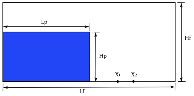
The model was set up according to an experiment that approximates the two-dimensional dam break (^{Zhou et al., 1999}), arranged as in Figure 3 in which the fluid is Hp = 600 mm deep and Lp = 1 200 mm long in a Lf = 3 220 mm long tank. The actual tank is 300 mm wide, which would be the absent dimension in the two-dimensional model. Clean water was considered under normal atmospheric conditions (temperature of 20ºC and pressure of 101.325 kPa) for the purposes of setting values for dynamic viscosity (μ = 0.001 Pa·s) and density (ρ = 998 kg/m³) of the fluid. Points X1 and X2 indicate the relative positions of depth sensors used in the physical experiment used as a calibration reference.

Figure 3 Setup geometry for two-dimensional dam-break over dry bed 

To assess the results, this case was solved with three different resolutions in a regular square arrangement: 800, 1 800 and 3 200 two-dimensional particles (particle size Δ x for each resolution is 30 mm, 20 mm and 15 mm respectively) for the fluid and a single layer of immobile virtual particles spaced at half the particle size for the tank boundaries. Smoothing length h was set at a constant 10 % greater than particle size Δ x . The artificial compressibility equation of state from (^{Monaghan, 1992}) was adopted with an artificial speed of sound of c ₀ equal to 80.0 m/s (a value used frequently in subsonic hydraulics cases when applying WSPH (^{Violeau, 2012})) since particle speeds expected are well under 10 m/s according to the experimental reference. This in turn helps reduce computational cost since the Verlet numerical stability criterion (^{Liu & Liu, 2003}) states that any Δt<Δx c0-1 can be chosen.

Dam break over wet bed. The case of conventional dam breaking does not allow the generation of wave dynamics to be verified until the movement of the fluid has led it to collide with some boundary, but this situation is very different from the dynamic condition in which a fluid is almost immobile and waves form before any boundary interactions occur or other forces are present other than those due to the inertia of the fluid. This distinct type of phenomena will happen in this second case, so a dam break over an existing, relatively long body of water was set up as a two-dimensional model based on a physical experiment with published data (^{Kocaman & Ozmen, 2015}) on water front position and photographs for some significant instants. The main purpose is to compare the formation of features such as wave fronts before any collision with a tank wall takes place.

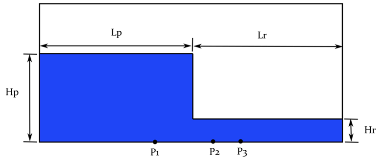
Following the description of the experiment and in accordance with the setup in Figure 4, two models were configured within the boundaries of a 9.0 m long, 0.6 m deep and 0.4 m wide tank. In both cases, the dam portion of fluid was Lp = 4.65 m long and Hp = 0.25 m deep. For the case of a shallow wet bed, a depth of Hr = 0.025 m was used, and the deeper wet bed had a depth of Hr = 0.10 m. The same density and viscosity for the previous test case were used here. Similar to the dry bed case, points P1, P2 and P3 indicate the relative positions of depth sensors used in the corresponding physical experiment used as a calibration reference.

Figure 4 Setup geometry for two-dimensional dam-break over wet bed 

The fluid was discretized in a regular Δ x particle size of 0.010 m, using 12 700 particles for the shallow bed case and 17 400 particles for the deeper bed case. The smoothing length, artificial compressibility, virtual boundary particles and time step size were chosen in the same way as in the previous test case.

Dam break

The model for the dam break was solved for the first 12 s after failure; regardless of the number of particles used, for times after t = 10 s the remaining velocities were small, and essentially hydrostatic equilibrium had been reached. During the highly dynamic stages, results are good in qualitative terms when compared with experimental profiles available in (^{Zhou et al., 1999}); the results given by Gap-SPH are shown in Figure 5 for different instants in dimensionless time gH-1, where H is the initial dam depth. In previous runs of this model, an increase from 800 to 1800 particles significantly changed the macroscopic behavior of the fluid, but a subsequent run with 3 200 particles did not show significant changes except for an improvement in the resolution of free surface artifacts, like the secondary wave seen at τ = 7.08 in Figure 5.

Figure 5 Numerical model profiles in time for dam break ( t < 2.2 s) 

To determine the quantitative validity of the results, instant depth data at positions X1 (2.25 m from the left boundary) and X2 (2.75 m from the left boundary) was obtained so as to compare it directly with experimental hydrographs available in (^{Zhou et al., 1999}) and the FVM modeling data of the same case using Fluent (a well-known commercial FVM software package) as presented by (^{Zhou et al., 1999}). As shown in Figures 6 and Figure 7, results calculated with GapSPH give a good match with both experimental data and the FVM model.

Figure 6 Hydrogram for position X1 = 2.25 m for 2D dam break 

Figure 7 Hydrogram for position X2 = 2.75 m for 2D dam break 

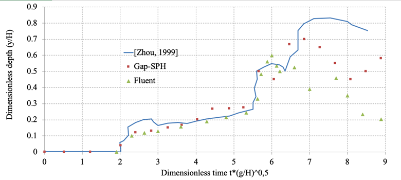
The FVM method is Eulerian, and therefore the driving equations are dependent upon a series of fixed nodes that form a mesh that must fill the continuum. In this type of cases, since there is a free surface, dynamic remeshing algorithms are required so that the FVM can handle the free boundary, which is in itself a challenge and a serious computational expense and may interfere with modeling accuracy. However, as mentioned above, mesh-based methods are very common in numerical modeling of fluid flow and both researchers and practitioners use results generated with the FVM as a benchmark to assess accuracy, efficiency and versatility of other methods. The numerical modeling by (^{Zhou et al., 1999}) for this case is shown here for that purpose. For an introductory discussion on the application of the FVM to computational fluid dynamics (^{Blazek, 2015}) is an appropriate starting point since it covers its mathematical formulation, commonly used algorithms, advantages and limitations, along with references to more detailed publications on the topic.

Before the first impact with the right boundary, the model implemented gives excellent coincidence except for the differences near the dimensionless time of τ = 1.75 (about 0.25 s after the beginning of movement) where the real fluid is deeper than predicted by numerical models. After the impact there is also a certain difference between the experiment and the model, but this is to be expected considering that the numerical model is for a single phase, so it does not reproduce the formation of foams or the effect of air bubbles. No turbulence models have been applied, and this contributes to differences in how much energy is dissipated during high shear conditions or direct impact with solid boundaries.

Regardless of the accuracy of the results, there is no evidence of instabilities or divergence of numerical origin in this case; additionally, as mentioned above, the fluid reaches a hydrostatic rest condition with small numerical oscillations in the order of magnitude of particle size.

Dam break over wet bed

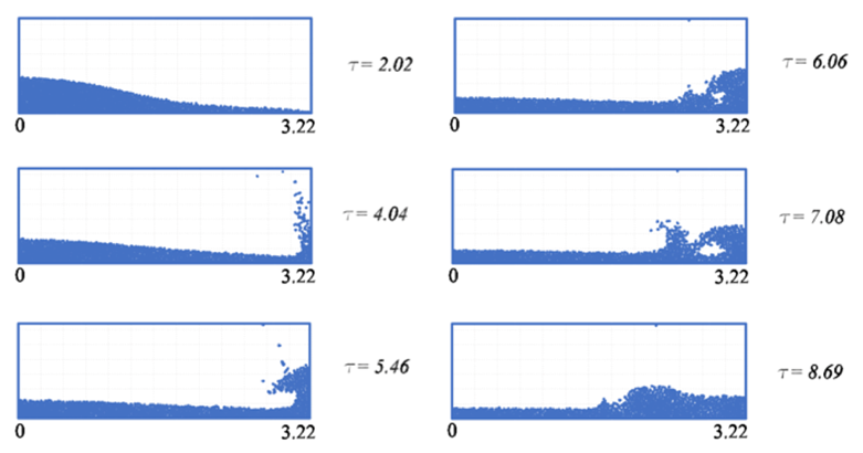
The numerical solutions for this case produced more complex dynamics, which is to be expected due to the presence of the downstream fluid. The models were solved only for the first 13 s (dimensionless time of about τ = 80) of behavior since for later times there are no available experimental data to compare with. Flow profiles are shown for several important instants in Figure 8 for both shallow and deep wet bed.

Figure 8 Depth profiles for dam break over wet bed 

If the photographs of the physical experiment, available in (^{Kocaman & Ozmen, 2015}), are used as a reference to determine the qualitative similarity of the flow condition, the shape and position of the waterfront coincide quite well, except for the appearance of a first concavity at t = 0.20 s in the case of shallow wet bed (Hr = 0.025 m, or α = 0.1); and that the wave crest is not well defined for t = 0.56 s in the case of the deeper wet bed (Hr = 0.100, or α = 0.4). Some lag of the numerical model with respect to the fluid is also present for some of the wave fronts.

To compare these results quantitatively, the experimental hydrographs for positions identified in the reference as P1, and P3; position P1 ( x = 4.4 m) is a point inside the dam, while position P3 ( x = 5.5 m) is a point close to the fall of the dam on the wet bed. The correspondence of the numerical model with the experimental data is shown in Figures 9 to 14.

Figure 9 Hydrograph at P1 for dam break over shallow wet bed (α = 0.1) 

Figure 10 Hydrograph at P1 for dam break over deep wet bed (α = 0.4) 

Figure 11 Hydrograph at P2 for dam break over shallow wet bed (α = 0.1) 

Figure 12 Hydrograph at P2 for dam break over deeper wet bed (α = 0.4) 

Figure 13 Hydrograph at P3 for dam break over shallow wet bed (α = 0.1) 

Figure 14 Hydrograph at P3 for dam break over deeper wet bed (α = 0.4) 

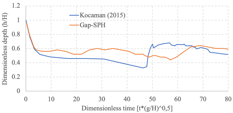
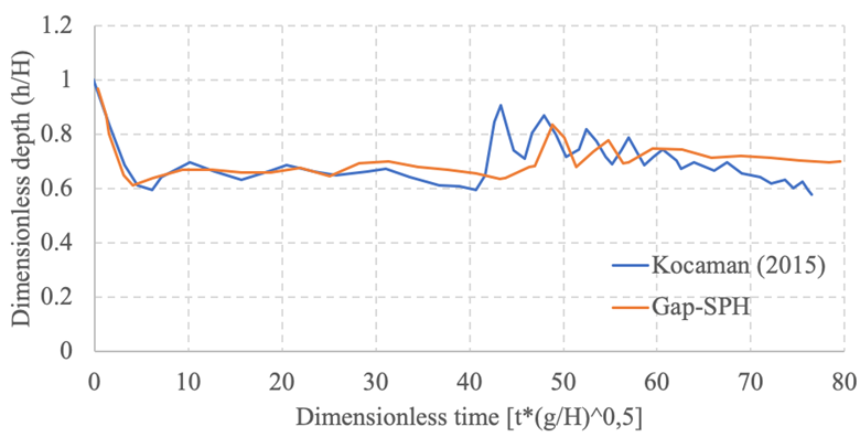
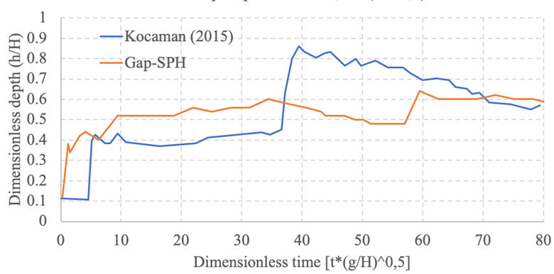
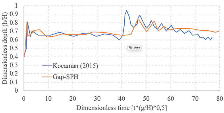
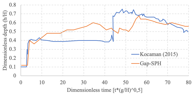
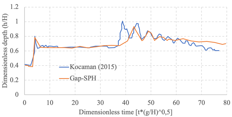
The results of the numerical model show good correspondence with the experimental measurements for the positions chosen for this comparison. The relative error is less than 12 % for α = 0.4 and less than 17 % for α = 0.1. The highest percentages of error occur at times and areas in which there are abrupt changes in the depth data, there is a frontal impact with a boundary or concave wave crests temporarily trap air inside. As shown in Figures 9 and 10, this is especially evident for point P1 of the case where the dam falls on a shallow bed (α = 0.1), which leads to the possibility that with higher resolution the accuracy could be improved.

In all cases, and probably not so closely related to resolution, the numerical model mostly shows a certain delay in the occurrence of the phenomena, but not in the speed of wave propagation as can be surmised by the delay between crests in Figures 12 and 14, which are the waves reflected by the right wall of the tank.

These processes also imply that a non-conservative dissipation of energy occurs in the numerical model that is not reflected in the experiment. That is unexpected since special turbulence models that can have this effect were not applied in these calculations. It is plausible that for future calibration cases certain empirical parameters of the numerical model will have to be adjusted, especially the empirical constants that direct the behavior of the virtual boundary particles. This would probably give better results than building a three-dimensional model with a comparable number of particles.

As with any numerical method, there are hundreds of examples that can be used as calibration cases and the effect of changing the parameters of the method needs to be checked before it can be categorically stated whether its accuracy is good for a certain field of application. The results in this study do not attempt to be complete in that sense, because the purpose of the process was to gain insight as to what effect do the fundamental definitions of the SPH have on general hydrodynamic problems and how it could be modified to better model hydraulics problems. As a response to this research objective, an outline of the related key findings can be found in the conclusion and future lines of development are suggested.