


 nova página do texto(beta)
 Inglês (pdf)
 Artigo em XML
 Referências do artigo
 Enviar este artigo por email
 Citado por SciELO
  Similares em
SciELO
Similares em
SciELO 
 Permalink
Introduction
Thermal comfort, according to ANSI/ASHRAE 55 (2017), is “that condition of mind that expresses satisfaction with the thermal environment and is assessed by subjective evaluation”, where the thermal perception basis is defined by physical and psychological sensations generated by the thermal environment stimuli, physical activity performed, experience and expectation. According to Humpreys & Nicol (1998), the adaptive approach is a way of studying thermal comfort; and it is methodologically supported as follows:
Subject is studied in his habitat, so the evaluation conditions vary continuously. In this sense, the studies are based on data collected in the field.
Human is considered as an active receptor in search of thermal comfort, so his physiological and psychological reactions are considered.
Thermal comfort conditions depend on the average outdoor temperature.
The dissemination of these studies commonly presents its findings based on the precise description of the methodology used and the detailed interpretation of the results obtained (Buonocore et al., 2020; Jindal, 2018; Mishra & Ramgopal, 2015; Rincón, 2019; González, 2012; Mayorga, 2012; Martínez, 2011; Bojórquez, 2010; Humpreys et al., 2007; Hernández & Gómez, 2007; Gómez et al., 2007a; García et al., 2005; Ambríz, 2005; Boerstra et al., 2002; Bravo & González, 2001; Auliciems, 1981; Auliciems & de Dear, 1998), but little is deepened on the procedure and methods used for the statistical processing of the data collected in the field, and less information is presented on the description of the different stages to which the data were submitted once collected: Since the database cleaning to achieve a consistent data set, up to the data correlation that allows for certainty of the results. Table 1 shows the common procedure to which the databases are statistically processed, in the different areas of knowledge, since they are collected in field studies.
Table 1 Statistics approaches for data analysis (Source: Made from Mishra, 2018)
| Data analysis | Techniques | Description |
|---|---|---|
| Filtering data | Pearson | Product moment correlation (r) |
| Kendall correlation & Spearman correlation | These are rank based correlations and would be strong for situations where the data is not linearly | |
| Data distribution | Shapiro-Wilk | Can be used for examining if a specific distribution is normal or not |
| One way ANOVA | Is used to determine whether there are any significant differences between the means of three or more independent variables (unrelated) | |
| Methods | Simple linear regression | Can quantifying the relationship between a dependent variable and an independent variable |
| Average by thermal sensation interval | Can quantifying the relationship between a dependent variable and an independent variable based on the average value of the comfort vote given It uses the descriptive statistics to estimate the neutrality value and two comfort ranges |
The document presents statistical alternatives that can be used for data processing collected in field from adaptive thermal comfort studies. Data processing is described in the following three stages:
Database capture.
Database preparation:
Outliers detection: Z-Score (Hernández et al., 2017; Nie et al., 1975), Quartile (Sánchez, 2007; NIST/SEMATECH, 2012) and Weighted Hierarchy (Rincón, 2019).
Omission of non-representative thermal sensation categories.
Omission of thermal sensation categories with the same value at physical variable.
Data correlation:
Simple linear regression (Cardona et al., 2013; Kelmansky, 2010; Martínez, 2005; Levin and Rubin, 2004).
Average by Thermal Sensation Intervals (Gómez et al., 2007b).
ANS/ASHRAE 55 (2017) method.
Although, the data correlation in this studies type can be carried out based on different statistical methods (Mishra, 2018; Humphreys et al., 2015), this document only describes those that are commonly used to analyze this phenomenon, as well as the method contained in the ANSI/ASHRAE 55 (2017). These statistical methods, of univariable type, focus on the correlation of an independent variable (physical variable recorded during the evaluation: Black globe temperature, dry bulb temperature, relative humidity and/or wind speed) and a variable dependent (comfort vote: Thermal sensation, thermal preference, hygric sensation, hygric preference, wind sensation, wind preference and/or personal acceptance) (Cardona et al., 2013; Martínez, 2005; Alegre & Cladera, 2002). With this, the data analysis does not make a difference in age, sex, level of clothing or activity level in the subjects analyzed, in order to estimate generic comfort models, although, if within the objectives of the research it is proposed to obtain specific indicators to any of the aforementioned anthropic variables, some selection filters would have to be applied during the data preparation stage.
Therefore, these data analysis methods could be used cautiously in any study on adaptive thermal comfort, regardless of the database size, including, the ASHRAE Global Thermal Comfort Database II (Luo et al., 2020; Ji et al., 2020; Wang et al., 2020; Földváry et al., 2018) or the use that various studies have made of this (Cheung et al., 2019).
It is worth mentioning that in recent years machine-learning algorithms have been presented as a new alternative for data analysis (Luo et al., 2020; Montazami et al., 2017) where the user explores complex data sets and searches for meaning among them, however, these are not the subject of this document due to the complexity and expertise required to program code that allow them function. However, there are studies (Luo et al., 2020; Loomans et al., 2020; Liu et al., 2019; Montazami et al., 2017) in which their operation has been explored in combination with the methods presented here, obtaining a 60 % mean certainty in the predicted results.
This paper is intended as a guide to the basic methods used for statistical processing of data collected in field studies.
Statistical data processing in adaptive thermal comfort studies
To obtain consistent results and carry out adequate data processing, the procedure is classified in three stages: a) Database capture, b) Database preparation, and, c) Data correlation.
Database capture
To use resources efficiently and structure an organized database, it is recommended that the questionnaire used to collect data contain a closed or mixed type question, predominantly, multiple choice and exclusionary questions (dichotomous or trichotomous) (Fernández, 2007). For do this, it is necessary to adopt a response system that allows the following characteristics:
Efficiency in electronic capture of responses.
Succession in the location of the answers written in the questionnaires.
Fast capture from a numerical coding of responses.
Ease of capture in multiple computer programs.
Reduction of errors in capturing responses.
The above is possible using a co-surveyed space format that allows the writing of the selected response. A co-surveyed space, according to Fernández (2007), is the individual area of each question in order to write the answer. The most practical is that each closed-type question has a rectangle located on the left side (Figure 1).
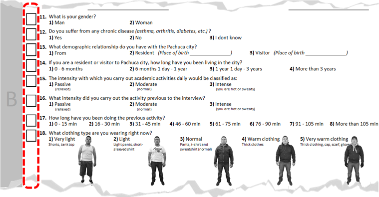
Figure 1 Trichotomic questions in which it is possible to observe the system of co-surveyed space. The questionnaire shows the single column of answers given by the subjects
The coding of each answering possibility from Arabic numbers is a characteristic that allows to facilitate the capture of data in computer, since in the keyboard the numbers are grouped progressively in a same strip or quadrant, therefore the time and errors decrease during this process, because only the left column is generated and captured by the total responses provided by the study subjects (Figure 1).
A conventional spreadsheet offers high performance and diversity of tools for capturing, manipulating, processing and generating data graphs, so it is suggested to use it in each of the stages mentioned. The table type format is commonly used to database capture; in this, each row represents an evaluation and each column represents an analyzed variable (CCPE, 2011).
Database preparation
Stage that allows giving a preventive treatment to the database in order to omit outliers that could affect the results sought. If this procedure is omitted, the results consistency due to the lack of treatment of erroneous data (bias) is jeopardized (CCPE, 2011). The purpose of this procedure is the review, validation and verification of the information consistency obtained in field, in order to get valid data that allow an accurate analysis of the given population reality.
Atypical data, also known as outliers, are observations that deviate from other observations that arouse the suspicion that they were generated by a different mechanism, are those extreme values of some variable that differ from the typical behavior of sample (Rodríguez et al., 2011; López, 2011), although, it is possible that these values are an indication that the data belong to a different population than the established sample, however, they are still considered outliers because they are not part of the value's regularity or homogeneity of most of the sample data. The consequences of an outlier can be serious and distort the results (inconsistency in accuracy) or affect the normality of database (data correlation/dispersion) (Hawkins, 1980).
According to Bisbé (2011), the outliers from a database can be treated in three ways: a) Substitution (replacement by specific or average value), b) Omission (keep the data but not use it for processing), and, c) Deletion (delete the value, the records are nullified). In this sense, for adaptive thermal comfort studies the omission, and not the elimination, of those values that could affect the results is recommended, since these could be useful at another time to achieve different research purposes. To do this, the steps for database cleaning are:
Outlier detection (data inconsistent with the group data homogeneity).
Omission of non-representative thermal sensation categories (less than 5.0 % of total observations collected).
Omission of thermal sensation categories with the same value at physical variable (only for the Averages by Thermal Sensation Interval method).
Outlier detection methods
There are various methods and procedures for treating the outliers; however, this document describes those used continuously in the different areas of knowledge: Z-Score and Cuartil (Hernández et al., 2017); additionally, a statistical basis method proposed by the authors of this paper is presented: Weighted Hierarchy.
Z-Score
According to Hernández et al. (2017), Z-Score method is the measure that indicates the direction and degree to which an individual value moves away from the mean, in a category of standard deviation (SD). Nie et al. (1975) mention that Z-score is commonly used to standardize the category of a variable measured at an interval level. Its formula is (1):
Where:
X = the score or value to transform
X̄ = the mean of the distribution to which the value to be transformed belongs
s = the standard deviation of the distribution to which the value to be transformed belongs, and z is the transformed value into standard deviation units
To use Z-score as a method to identify outliers, it is necessary that each value of the distribution be in the range -3.0 SD to +3.0 SD (López, 2011).
As an example, Table 2 shows the thermal sensation (TS) data collected, where the TS category used was from 1 to 7 based on the seven points of thermal perception suggested in ANSI/ASHRAE 55 (2017).
Table 2 Outliers’ identification based on the Z-Score method
|
|
|
|
|---|---|---|
| 5 | 1.76 | Non-outlier |
| 4 | 0.79 | Non-outlier |
| 4 | 0.79 | Non-outlier |
| 4 | 0.79 | Non-outlier |
| 4 | 0.79 | Non-outlier |
| 4 | 0.79 | Non-outlier |
| 4 | 0.79 | Non-outlier |
| 4 | 0.79 | Non-outlier |
| 4 | 0.79 | Non-outlier |
| 3 | -0.18 | Non-outlier |
| 3 | -0.18 | Non-outlier |
| 3 | -0.18 | Non-outlier |
| 3 | -0.18 | Non-outlier |
| 3 | -0.18 | Non-outlier |
| 3 | -0.18 | Non-outlier |
| 3 | -0.18 | Non-outlier |
| 3 | -0.18 | Non-outlier |
| 2 | -1.16 | Non-outlier |
| 2 | -1.16 | Non-outlier |
| 1 | -2.13 | Non-outlier |
| 1 | -2.13 | Non-outlier |
Sample column contains the TS categories chosen by the subjects during the evaluation, Z-Score column shows the SD of each of the values concentrated in the previous column, and Is it an outlier? column, specify if the value is outlier; this, from Z-Score with an interval of -3.0 SD to +3.0 SD. In this case, none of the records collected (with TS categories from 1 to 5) are considered outliers.
Quartile
According to Sánchez (2007), quartiles are the three statistical measures of position that have the property of dividing the dataset in four equal portions:
The first quartile Q1 splits off the lowest 25 % of data distribution from the highest 75 %.
The second quartile Q2, cuts dataset in half; is the equivalent to the dataset median.
The third quartile Q3 splits off the highest 25 % of data distribution from the lowest 75 %.
The general quartile formula for grouped data is (2):
Where:
L i = the lower limit of the quartile class
k = the quartile
n = the observations number
Ma = the absolute frequency immediately below the quartile class
w = the width of the class containing the quartile
mc = the frequency of the class containing the quartile
NIST/SEMATECH (2012) mentions that to use Quartile as a method to identify outliers, it is necessary to calculate the interquartile range (IQ) -difference between the upper quartile Q3 and the lower quartile Q1-, then, continue with the following premises:
Very outlier. When the analyzed data has a value greater than Q3 + 3.0 IQ (MaLs) or a value less than Q1 - 3.0 IQ (MaLi).
Slightly outlier. When the analyzed data has a value greater than Q3 + 1.5 IQ (AaLs) or a value less than Q1 - 1.5 IQ (AaLi).
Non-outlier. When the analyzed data has a value between AaLi and AaLs.
Following the example of the previous section, the Table 3 shows Sample column containing the TS categories chosen in the thermal comfort study, Very outlier column shows the MaLi and MaLs limits, Slightly outlier column shows the AaLi and AaLs limits, and, Is it an outlier? column defines whether each value contained in the first column is or is not outlier (very outlier or slightly outlier) depending on the value with respect to the limits defined in the two previous columns. According to this method, only records with the TS category equal to 1 are slightly outlier, since their numerical value is less than 1.5.
Table 3 Outliers’ identification based on the Quartile method
| Sample (TS category) | Very outlier (MaLi-MaLs) | Slightly outlier (AaLi-AaLs) | Is it an outlier? (AaLi>value>AaLs) |
|---|---|---|---|
| 5 | 0.0 - 7.0 | 1.5 - 5.5 | Non-outlier |
| 4 | 0.0 - 7.0 | 1.5 - 5.5 | Non-outlier |
| 4 | 0.0 - 7.0 | 1.5 - 5.5 | Non-outlier |
| 4 | 0.0 - 7.0 | 1.5 - 5.5 | Non-outlier |
| 4 | 0.0 - 7.0 | 1.5 - 5.5 | Non-outlier |
| 4 | 0.0 - 7.0 | 1.5 - 5.5 | Non-outlier |
| 4 | 0.0 - 7.0 | 1.5 - 5.5 | Non-outlier |
| 4 | 0.0 - 7.0 | 1.5 - 5.5 | Non-outlier |
| 4 | 0.0 - 7.0 | 1.5 - 5.5 | Non-outlier |
| 3 | 0.0 - 7.0 | 1.5 - 5.5 | Non-outlier |
| 3 | 0.0 - 7.0 | 1.5 - 5.5 | Non-outlier |
| 3 | 0.0 - 7.0 | 1.5 - 5.5 | Non-outlier |
| 3 | 0.0 - 7.0 | 1.5 - 5.5 | Non-outlier |
| 3 | 0.0 - 7.0 | 1.5 - 5.5 | Non-outlier |
| 3 | 0.0 - 7.0 | 1.5 - 5.5 | Non-outlier |
| 3 | 0.0 - 7.0 | 1.5 - 5.5 | Non-outlier |
| 3 | 0.0 - 7.0 | 1.5 - 5.5 | Non-outlier |
| 2 | 0.0 - 7.0 | 1.5 - 5.5 | Non-outlier |
| 2 | 0.0 - 7.0 | 1.5 - 5.5 | Non-outlier |
| 1 | 0.0 - 7.0 | 1.5 - 5.5 | Slightly outlier |
| 1 | 0.0 - 7.0 | 1.5 - 5.5 | Slightly outlier |
Weighted Hierarchy
Z-Score and Quartile methods determine the outliers of a data universe from the distance that its value represents with respect to the normal distribution of the records; however, based on the TS subjective categories on which the phenomenon of thermal comfort is supported (ANSI/ASHRAE 55, 2017), the criteria established in this method to identify the presence or absence of outliers in a database, are:
The perceptual meaning that represents each of the values used in the TS subjective category to evaluate the environment acceptance conditions and, not so, the numerical value interpreted by Z-Score and Quartile in each TS category.
The frequency with which each TS category is chosen under the same, or similar, magnitude of physical variable (set of observations generated at different moments close to each other) and the proportion that each of them represents with respect to the total opinions collected.
In other words, the Weighted Hierarchy method bases its criterion of outliers’ identification on the meaning, frequency and proportional representation of each TS category, and not on the numerical value that each one represents.
This method is based on the statistical measure of the proportion, also known as relative frequency, which, according to Ruíz (2004), is a summary measure consisting of the number of times a value is presented with respect to the total sample; this statistical measure has the advantage of being applied in qualitative variables. Its general formula is (3):
Where:
n i = the observations of interest (number of times the same value is repeated in the sample)
n = the sample size (total number of observations)
P i = the weighted proportion representing the value with respect to the total number of observations
So that the proportion to be applied as a method of identifying outliers, some adjustments must be made and some application conditions clarified:
The values used to describe the sample data are from 1 to 7 (adaptation of TS scale contained in ANSI/ASHRAE 55 (2017), 1 = Cold and 7 = Hot).
The criterion adopted to determine outliers is to obtain a value of less than 0.1429 (1/7 of the total sample size) when applying the proportion equation to each observation set that have chosen the same TS category. This based on the assumption that, under hypothetically homogeneous conditions, the minimum number of subjects that has chosen each of the seven TS categories is 1/7 of the studied sample.
Outliers’ identification is realized from an evaluations series carried out in close proximity to each other, whose magnitude of the physical variable is the same or similar between them. This allows to identify quickly, efficiently and accurately, the atypical observations, e.g.
Following the example of the previous sections, the Table 4 shows the Sample column containing the TS categories chosen in the thermal comfort study; Proportion column shows the proportion that each of these categories represents with respect to the observations total, and the Is it an outlier? column defines, from a value less than 0.1429 in the Proportion column, if each value of the first column is an outlier.
Table 4 Outliers’ identification based on the Weighted Hierarchy method
| Sample (TS category) | Proportion (Pi= xi /n) | Is it an outlier? (Pi < 1/7) |
|---|---|---|
| 5 | 0.05 | Outlier |
| 4 | 0.38 | Non-outlier |
| 4 | 0.38 | Non-outlier |
| 4 | 0.38 | Non-outlier |
| 4 | 0.38 | Non-outlier |
| 4 | 0.38 | Non-outlier |
| 4 | 0.38 | Non-outlier |
| 4 | 0.38 | Non-outlier |
| 4 | 0.38 | Non-outlier |
| 3 | 0.38 | Non-outlier |
| 3 | 0.38 | Non-outlier |
| 3 | 0.38 | Non-outlier |
| 3 | 0.38 | Non-outlier |
| 3 | 0.38 | Non-outlier |
| 3 | 0.38 | Non-outlier |
| 3 | 0.38 | Non-outlier |
| 3 | 0.38 | Non-outlier |
| 2 | 0.10 | Outlier |
| 2 | 0.10 | Outlier |
| 1 | 0.10 | Outlier |
| 1 | 0.10 | Outlier |
This procedure allows to obtain greater consistency in the outliers’ classification, therefore, it determines that the TS categories that only have one or two responses (categories 1, 2 and 5) are atypical with respect to the total observations collected, which allows data processing only with the observations of the TS categories that reflect the highest frequency (categories 3 and 4).
Omission of non-representative thermal sensation categories
It refers to the non-consideration of those observations of a same TS category that don’t represent even 5.0 % of observations collected throughout the study period. The foregoing indicates that, unlike the outliers’ omission that is carried out by a set of observations collected in close moments with each other, the omission of non-representative TS categories is applied per study period.
Percentage value derives from the confidence interval commonly used in the different areas of knowledge for the design of population sample, so it can be considered as the buffer interval that allows defining the level of confidence (certainty) with which it would be presumed that the answers given by the evaluated sample would be entirely based on the recorded magnitude of the analyzed variables (Creative Research Systems, 2010).
It is worth mentioning that this filter does not always represent a benefit in the expected results, therefore, while with Average by Thermal Sensation Interval method the coefficient of determination (r 2 ) is increased, with Simple Linear Regression method the coefficient of determination usually decreases.
Omission of thermal sensation categories with same value at physical variable
As anticipated, this filter only applies to Averages by Thermal Sensation Interval method (ATSI; or, MIST for its acronym in Spanish), because it is the one that uses the standard deviation to estimate comfort ranges.
According to Ruíz (2004), the standard deviation (SD) is the measure of the degree of dispersion of a data set with respect to its average value; it is defined as the square root of the variable’s variance and can be significantly influenced by outliers. To calculate the SD it is necessary to have a dataset of at least two values.
In adaptive thermal comfort studies, some extreme TS categories (1, 2, 6 and/or 7 of the TS scale) may have equal or close values in the magnitude of the physical variable recorded, by virtue of being carried out in immediate evaluation moments throughout the study period, so that the oscillation of this variable is null or reduced. In this sense, with the use of ATSI, the above scenario implies certainty in the neutral value; not so, in that of the comfort ranges, since, it is impossible to calculate any SD that allows obtaining the linear regressions of which these values are defined. Although the linear regression of the means is consistent, the linear regressions of the comfort ranges are affected by the equality or proximity presented by the magnitude of the physical variable, which results in a decrease in the coefficient of determination for these latter cases.
Therefore, it is suggested to omit the TS categories with the same or close magnitude in physical variable, in order to avoid inconsistencies or possible errors of interpretation in the results.
Data correlation
To carry out the correlation and data analysis, two statistical methods of univariate correlation are described, and a method of ANSI/ASHRAE 55 (2017):
Simple Linear Regression method (Cardona, 2013; Kelmansky, 2010; Martínez, 2005; Levin & Rubin, 2004).
Average by Thermal Sensation Intervals method (Gómez et al., 2007b).
ANSI/ASHRAE 55 (2017) method.
Simple Linear Regression method
Linear regression is a statistical technique used to identify the relationship between variables. It is used in social research to predict a phenomenon, from economic measures to different aspects of human behavior.
According to Cardona et al. (2013) simple linear regression (SLR) allows quantifying the relationship between a dependent variable (Y, endogenous or criterion) and an independent variable (X, exogenous or predictor), exposing it in a linear equation that allows predicting the relationship. It is about finding the middle line that synthesizes the dependence between the variable Y and the X, in order to explain the cause of the dependent variable and predict the future values of Y for values given in X (Martínez, 2005).
Relationship between the two variables is described by the linear Equation (4) (Kelmansky, 2010):
Where:
α + βx = the unknown parameters to estimate
ϵ = the error in predicted parameters
y = the variable to predict
The dependent variable Y is linearly related to the independent variable X, plus an error that addresses the variability in Y that cannot be explained with the linear relationship. Cardona et al. (2013) mention that there are measures to determine the degree of relationship between the two variables: Coefficient of determination (r 2 ) and correlation coefficient (r).
Coefficient of determination is a standardized measure that indicates the relationship between the two variables in 0 to 1 range; 0 means total independence between the variables and 1 means the perfect relationship between them (Kelmansky, 2010; Martínez, 2005; Levin & Rubin 2004). Based on Kelmansky (2010), the general Equation (5) of r 2 can be expressed as:
Where:
Numerator = variation explained
Denominator = total variation
r 2 = coefficient of determination
A typical error in the interpretation of r 2 is the lack of consideration of the sample size, which usually varies inversely. It is enough to consider a small number of observations so that r 2 gets a value close to 1, without evidencing the existence of a marked linear relationship between two variables (Martínez, 2005).
On the other hand, correlation coefficient is a measure used to describe how one variable explains to the one (Cardona et al., 2013). It is expressed as the square root of the coefficient of determination (6):
Where:
(b sign) = the b sign according to direct (+) or inverse (-) relationship
r 2 = the coefficient of determination, and r is the correlation coefficient
Correlation coefficient measures the relationship intensity between the two variables in -1 to 1 range; in both cases there is an intense relationship, negative and positive respectively, as the value approaches to 0, the relationship weakens until it is lacking (Cardona et al., 2013). In adaptive thermal comfort studies, the dispersion diagram is made up from the data pairs collected in the site evaluations: Independent variables are the physical variables recorded (WBT, BGT, RH and WS) and dependent variables are TS votes given by the study subjects. The dispersion diagram is generated from TS votes on Y axis and physical variables on X axis (Kelmansky, 2010).
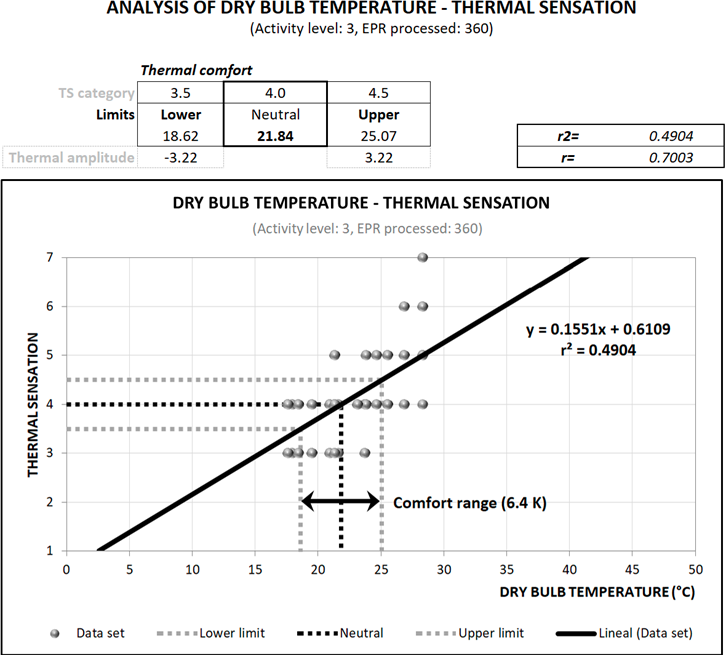
Thermal comfort studies objective is not to know the TS response of study subjects from certain environmental physical conditions, but to estimate the thermal comfort from each of the physical variables that intervene in the subjects thermal perception, so it is advisable clear to X from the linear function obtained by the regression line and substitute to Y for a value equal to 4 (TS category equivalent to neutral level) to obtain the comfort value of the physical variable analyzed. Likewise, to estimate the comfort range limits, Y must be substituted for 3.5 and 4.5 according to González & Bravo (2003), or, 3.0 and 5.0 according to Fanger (1972) (Figure 2).
Some advantages of using this statistical method are:
Estimation of a neutral value and a comfort range.
Statistical consistency in the correlation of any physical variable registered with the perceived TS, to estimate the neutral value and comfort ranges. However, this consistency is reduced if the correlation is made with comfort votes other than the TS, e.g.: Hydric sensation, thermal preference, hydric preference, wind sensation, wind preference and personal acceptance.
Likewise, the disadvantages of using this statistical method are:
Comfort range estimate is at the analyst's criteria and is usually modeled equidistant to the comfort value.
Coefficient of determination value is below 0.5, which, in thermal comfort studies, corresponds to a low correlation and a high dispersion in the sample.
Averages by Thermal Sensation Interval method
This statistical method was proposed by Gómez et al. (2007b), based on Nicol's (1993) proposal for asymmetric climates, where the thermal comfort range limits aren't equidistant to neutral temperature. The method consists in using the descriptive statistics to estimate the neutrality value and the comfort ranges of the physical variable analyzed from the comfort votes expressed by the study subjects. In Figure 3 a general diagram of the data processing can be seen from the use of the mentioned method.
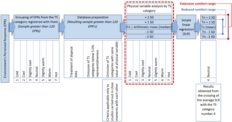
Source: Own elaboration based on Bojórquez, 2010
Figure 3 General diagram of the data processing based on the ATSI statistical method
According to this diagram (Figure 3), the procedure that describes each of the stages is as follows:
Conformation of a database from the values obtained in field. Each data pair consisting of a comfort vote and a physical variable magnitude, it can be identified interchangeably as Observation or Environment's Perceived Response (EPR).
Grouping of EPRs from the TS category registered. According to Gómez et al. (2009) and Bojórquez (2010), it is recommended that at least 120 observations be collected each study period in order to get sufficient statistical consistency in data processing.
Database preparation: a) Treatment of outliers, b) omission of TS categories below 5.0 % representativeness, and, c) omission of TS categories with same value at physical variable.
From the physical variable values grouped by TS category, the arithmetic mean is calculated, which, when is plotted with the corresponding TS category, forms the necessary dispersion diagram to generate the linear regression (average SLR) which allows to estimate the neutral value (Figure 4).
From the physical variable values grouped by TS category, the SD is calculated (Figure 4).
For each ST category, add and subtract one SD (± 1 SD) from the arithmetic mean. The values obtained, together with the ST category to which they belong, make up the dispersion diagram that generates the linear regression SLR (1 ± SD) with which the reduced comfort range limits are estimated. The procedure is repeated with the addition and subtraction of two SD (± 2 SD) to form the dispersion diagram with the linear regression (SLR ± 2 SD) that estimates the extensive comfort range (Figure 4).
Estimation of neutral value and comfort ranges as follows:
Neutral value = Abscissa resulting from the crossing of the average SLR with the TS category number 4.
Reduced comfort range's upper limit = Abscissa resulting from the crossing of the SLR + 1 DS with the TS category number 4.
Reduced comfort range's lower limit = Abscissa resulting from the crossing of the SLR - 1 DS with the TS category number 4.
Extensive comfort range's upper limit = Abscissa resulting from the crossing of the SLR + 2 DS with the TS category number 4.
Extensive comfort range's lower limit = Abscissa resulting from the crossing of the SLR - 2 DS with the TS category number 4.
According to Reynaga (2011), for normally distributed data, the range of ± 1 SD includes 68.26 % of the answers given by the study subjects, the range of ± 2 SD includes 95.45 % of them, and, the range of ± 3 SD includes 99.74 % (Figure 5). For non-distributed data, this percentage may vary, so it is recommended to obtain as many responses as possible in field studies to get a normal distribution.
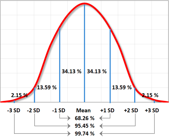
Source: Own elaboration based on Reynaga, 2011
Figure 5 Standard deviation ranges for normally distributed data
8. Obtaining the coefficient of determination (r 2 ) and the linear equation (y = α + βx) of each SLR generated, in order to validate the correlation between the two variables. According to Bojórquez (2010), the certainty of this method is based on the value obtained in r 2 of the average SLR (Figure 4).
In this studies type it is common that the analyzed sample to be obtained from a statistical design applied to the target population, so the amount of observations obtained consistently represents it. In this sense, Bojórquez (2010) mentions that r 2 is the one who identifies the dispersion degree of the TS responses given with respect to the physical variables recorded; therefore, based on different authors (Gomez et al., 2009; Humphreys et al., 2007; Ruíz, 2007; Nikolopoulou, 2004; Bravo & González, 2003; de Dear et al., 1997; Nicol et al., 1993; Auliciems, 1981; Humphreys, 1976; Bedford, 1936), the following criteria are established to determine the relationship degree between the variables:
If r 2 ≥ 0.9 the correlation is very high, so there is certainty in the responses concentration; If 0.7 ≤ r 2 <0.9 the correlation is high, the sample is poorly dispersed.
If 0.5 ≤ r 2 <0.7 the correlation is mean, the sample has a moderate concentration.
If r 2 < 0.5 the correlation is low, with a high dispersion degree in the sample.
9. Phenomenological (or circumstantial) analysis of each value obtained, from the graphic and matrix resources generated with this method, in order to visualize and substantiate the thermal adaptation that the studied sample achieves in each evaluation period.
In asymmetric distributions, it is recommended to use the median and, therefore, add or subtract the SD from it (Bojórquez, 2010).
According to recent thermal comfort studies (Rincón, 2019; González, 2012; Martínez, 2011; Bojórquez, 2010; Gómez et al., 2007a; Hernández & Gómez, 2007), the advantages identified with the use of ATSI method are:
Greater consistency in the results obtained and a coefficient of determination close to the unity.
A neutral value and two comfort ranges are estimated:
Comfort ranges are not generally equidistant to neutral value, adapting more precisely to the environmental conditions given in the study place. This characteristic differs from that observed with the linear regression method, where the comfort range is equidistant to neutral value.
The average SLR's r 2 is usually close to unity, which allows, according to Bojórquez (2010), to be certain of the degree of relationship between both variables.
A phenomenological interpretation can be obtained from the five SLRs generated; for example, when the r 2 value is higher in the lower limits of the comfort ranges, greater human adaptation to thermal conditions below the neutral value can be interpreted. Additionally, from the dispersion diagram it can be interpreted that the closer the data pairs are plotted by TS category, is lower the human adaptation, and, the greater the dispersion, is greater the human adaptation.
Neutral value estimated with this method is very close to neutral temperature (Tn) obtained with the Auliciems & Szokolay’s (1997) linear equation, which allows bioclimatically validating the result, unlike that obtained with the simple linear regression method, which usually results in a significant thermal difference from the reference cited.
However, the disadvantages that this method presents are:
The five SLRs obtained are the product of a reduced data set (maximum seven pairs of data, the equivalent to the seven TS categories), so the value of their r 2 is close to the unity.
Linear regression is not always adequate to plot the SLR ± 1 DS and/or ± 2 DS, since sometimes a clear curve trend can be observed between the plotted dispersion points, indicating that some other regression type should be used.
When in a TS category the physical variable magnitudes are close to each other or have the same value (usually in the extreme TS categories), the dispersion diagram usually alters the regression lines significantly and, consequently, the expected results.
The main difference between the ATSI method and SLR method is that, before obtaining the regression line that characterizes the studied sample, the EPRs that coincide in a TS category are grouped in order to calculate the arithmetic mean and the standard deviation of the physical variable magnitudes. Thus, linear regression does not derive from all the sample data pairs, but only from the mean values (and the addition and subtraction of one and two SD) from each TS category involved in the analysis.
ANSI/ASHRAE 55 method
This method is only valid for naturally ventilated indoor spaces, where subjects carry out sedentary activities (1.0 met to 1.3 met) and have the possibility of adapting their clothing and immediate environment (from the closing or opening of windows, e.g.) to solve the thermal needs of their space (ANSI/ASHRAE 55, 2017).
It is based on a thermal comfort diagram defined for study cases with similar characteristics to those mentioned above (Figure 6). In it, the outdoor ambient temperature (abscissa) and the indoor operative temperature (ordinate) are plotted to know if the study subjects are in thermal comfort conditions.
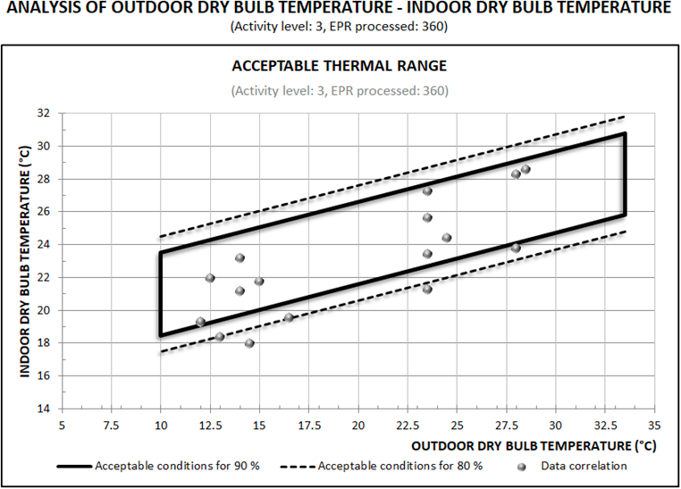
For this, the diagram allows to visualize, from two thermal comfort zones, the permissible temperature for indoor spaces: The first marks the acceptable conditions for 80.0 % of the subjects and, the other, for 90.0 % from them. The limits that define the first zone are for everyday applications and should be used when there is no additional information available; meanwhile, it is possible to use the limits of the second zone when more precise thermal comfort is desired (ANSI/ASHRAE 55, 2017).
Comfort range is plotted at ± 3.5 °C of the neutral value for 80.0 % acceptance, and at ± 2.5 °C for 90.0 % acceptance. To avoid uncertainty in the results obtained, it's invalid to extrapolate the permissible temperature limits to areas outside the marked limits.
The diagram considers the adaptation of people's clothing in naturally conditioned spaces to relate the indoor thermal comfort range with the outdoor climate, so it isn't necessary to estimate the clothing values used in the space. Similarly, the relative humidity and wind speed limits aren't necessary with the use of this method.
Results
The three methods presented in this document were applied to a specific case study in order to find the particularities that each one offers both in the data correlation stage, and in the estimation of results, so the values below presented (neutral temperature and thermal comfort ranges) should only be considered as references for this purpose.
Case study was in Pachuca city, Hidalgo, whose bioclimate is semi-dry, with an annual temperature of 14.3 °C, an annual relative humidity of 62.6 % and an average wind speed of 2.7 m/s from the N and NE (Rincón, 2019). Study sample was young adults between 15 and 24 years old, residents of Pachuca city, with predominantly sedentary physical activity (1.2 met, according to ISO 8996, 2004), moderate clothing (1.0 clo, according to ANSI/ASHRAE 55, 2017) and active attitude to solve their thermal requirements in naturally ventilated buildings. The statistical analysis was applied to the thermal transition between the cold and warm periods of this city.
With SLR method a comfort temperature of 21.8 °C and a thermal comfort range of 18.6 °C to 25.0 °C were obtained, equivalent to equidistant thermal amplitude of ± 3.2 K (see Figure 2). According to Bojórquez (2010), the correlation is low because the r 2 was 0.49, since with this method all data pairs of the linear regression from which is obtained both neutral temperature and comfort thermal range are considered. To estimate these results, the outliers were omitted with the Weighted Hierarchy method, so that of 397 EPRs collected; only 360 EPRs were processed (Figure 7).
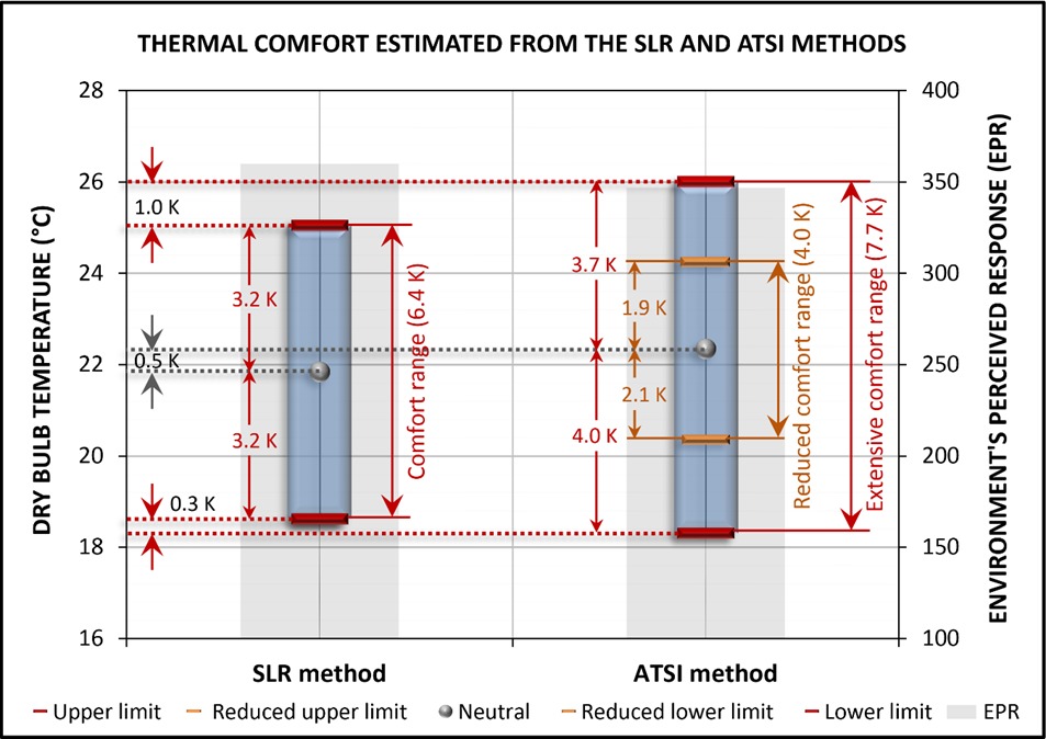
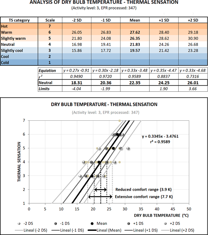
With ATSI method, the neutral temperature was estimated at 22.3 °C with a reduced comfort range of 20.4 °C to 24.2 °C and an extensive comfort range of 18.3 °C to 26.0 °C; in both cases, the amplitude was not equidistant to neutral temperature, with -2.1 K and +1.9 K for reduced range and -4.0 K and +3.7 K for extensive range (see Figure 4). As can be seen, numerically and graphically, the amplitude show to greater psychophysiological adaptation to temperatures below neutral than at temperatures above this; natural characteristic in human adaptation according to hygrothermal conditions present in the study period (thermal transition period) and subjects thermal history when leaving the cold period and approaching the warm period. According to Bojórquez (2010), the correlation is very high because the r 2 was 0.96, a value above that obtained with the SLR method, since in this case, r 2 is obtained from a reduced data set that is generated with the unique data pair presented by each TS category involved in statistical analysis. To estimate these results, the outliers were omitted with the Weighted Hierarchy method, as well as the TS categories with representativeness below 5.0 % of the total EPR, so from 397 EPRs collected, only 347 EPRs were processed (Figure 7).
Figure 7 shows the thermal comfort values estimated from the RLS and ATSI methods; here you can see the thermal differences obtained depending on the analysis method used.
With the ANSI/ASHRAE 55 (2017) method it was only possible to determine, based on the evaluation thermal conditions, whether the subjects were in thermal comfort according to the pre-established areas in the diagram. With this, in Figure 6 it is possible to observe that a significant percentage of subjects evaluated were in thermal comfort, some close to the range lower limit that determines the acceptable conditions for 80.0 % of subjects.
The points plotted to the left of the diagram correspond to the subjects evaluated in the morning, while the points plotted to the right of the diagram correspond to those evaluated in the evening; this is why the dispersion diagram is fragmented at both ends. To analyze the data with this method, the outliers were omitted with the Weighted Hierarchy method, so that of 397 EPRs collected; only 360 EPRs were plotted.
Discussion
With SLR method, the comfort range amplitude is usually equidistant to the neutral temperature by the analyst's criteria, since the thermal range limits are obtained with the crossing of the regression line and the values 3.5 and 4.5 on the ordinates (González & Bravo, 2003). In this case, the data correlation is usually low (Bojórquez, 2010) because the linear regression is obtained from the complete data set.
On the other hand, with ATSI method is possible to notice, firstly, the estimation of two thermal comfort ranges, subsequently, the possibility of a phenomenological interpretation depending on the causal disposition of each generated linear regression. In this case, the data correlation is usually very high (0.9< r 2 <1.0, according to Bojórquez, 2010) because each linear regression is obtained from a maximum set of seven pairs of data.
SLR and ATSI methods allow correlating any comfort vote collected in the field studies with any thermal environment physical variable recorded simultaneously; that is, with both methods, the sensation and preference (thermal, hygric and wind, as well as personal acceptance of space and mood derived from environmental conditions) obtained as part of the thermal environment’s subjective perception, can be correlated individually and interchangeably with each of the physical variables recorded during the evaluation (dry bulb temperature, black globe temperature, relative humidity, wind speed and any recorded variable of the thermal environment), in order to find the degree of association and dependence between both variables and explain the influence of one with respect to the other.
Regarding the ANSI/ASHRAE 55 (2017) method, it is only possible to correlate two physical variables of the thermal environment (one indoor and one outdoor), because the thermal comfort range is already defined for specific study cases: Naturally ventilated indoor, where subjects carry out sedentary activities (1.0 met to 1.3 met) and have the possibility of adapting their clothing level and immediate environment (from the closing or opening of windows, e.g.) to solve their thermal requirements. With this method it is not possible to estimate the neutral temperature and the thermal comfort range; however, it allows the possibility of knowing if the studied sample is in thermal comfort, or not, from the comfort zone previously defined. Based on the comfort zone shape, it is possible to notice a range of comfort equidistant to neutral temperature, since the comfort zone cross section is uniform along its length.
As a complementary resource to this paper, a personalized spreadsheet that allows the correlation of the data pairs collected in field studies (comfort vote and registered physical variable) from the statistical methods described above is attached, so that another researchers related to this topic can used it extensively in their studies. The personalization of the spreadsheet is based on Visual Basic programming that allows, in addition to processing the data with a couple of clicks, to offer numerically and graphically the neutral value and comfort ranges, according to the variables selected to statistically process the data. Derived from the country where the spreadsheet was developed (Mexico), the presentation language is Spanish. The database, the estimated values and the graphs presented, correspond to the case study described in the results.
Conclusions
The procedure presented is based on statistical methods or models already established and used in different areas of knowledge. Undoubtedly, there are numerous procedures to statistically process a database; however, the one presented here adapts more flexibly to adaptive thermal comfort studies.
According to different thermal comfort studies (Rincón, 2019; González, 2012; Martínez, 2011; Bojórquez, 2010, Gómez et al., 2009; Gómez et al., 2007a; Gómez et al., 2007b; Hernández & Gómez, 2007; Ruíz, 2007), it is possible to identify that the ATSI method, proposed by Gómez et al. (2007b), offers results with greater consistency regarding the thermal sensation and subjects personal behavior, because its causal and phenomenological correspondence with the hygrothermal conditions presented during the evaluation. This consistency is observed with the values obtained in the coefficient of determination and the slope of the line. In addition, with the ATSI method it is possible to estimate the neutral value and two comfort ranges (extensive and reduced) of the analyzed physical variable that, not necessarily, are equidistant from the neutrality value (Bojórquez, 2010).
In this sense, the SLR method also allows estimating the neutral value of the analyzed variable and a comfort range, however, the latter is at the analyst's criteria and is usually modeled equidistant from the neutral value. On the other hand, with the ANSI/ASHRAE 55 (2017) method it is not possible to estimate thermal comfort from data collected in the field, it is only possible to know if the study subjects are, or not, in thermal comfort conditions.
In addition, it was observed that the values estimated with the ATSI method are consistent regardless of the comfort vote and the correlated physical variable, while with the other methods, the consistency of the results is limited only to the thermal analysis. Another advantage of the ATSI method is that the comfort ranges limits are not necessarily equidistant from the neutral value; these are periodically adjusted based on the acclimatization that individuals adopt throughout the year. This is probably due to the phenomenological effect that it is possible to represent and interpret with this method, when estimating the comfort ranges with the addition and subtraction of standard deviations who consider the representativeness of the different manifestations of environmental adaptation that the subjects have against the changing conditions of the thermal environment.

