


 text new page (beta)
 English (pdf)
 Article in xml format
 Article references
 Send this article by e-mail
 Cited by SciELO
  Similars in
SciELO
Similars in
SciELO 
 Permalink
Introduction
Transportation systems are vital for the economies of the world and over the years it has been recognized that it is important to understand and model the behavior of these systems; these requirements are important for designing better transport systems for goods and passengers (Möller, 2014).
In Mexico the first railway line was inaugurated in 1872 and connected Mexico city with the port of Veracruz, passing through Orizaba city; since then, the Mexican railroad has been an important transport system in the modern history of the country, to the extent that its performance is critical for the development of the Mexican economy since it is the central axis for the development of efficient supply chains for the industrial sector, in addition Mexican railroads transport most of the grain consumed in the country.
The Mexican rail network is denser (measured in km-route / million km2) than the networks of countries such as China and Russia (the busiest in Asia and Europe) and Brazil (the busiest in Latin America) (OCDE, 2014).
The railroad has been used mainly for the transport of raw materials such as coal and iron ore; these are abundant in China and Russia where the railways are mainly focused on moving these products; in Mexico, the sources of these raw materials are less abundant; however, it is considered that the Mexican rail system is a general cargo transport; in general cargo systems there is a greater diversity of products, with multiple origins and destinations (OCDE, 2014). In 2017, the total cargo volume was 126.9 million tons; industrial products accounted for 47.1 % of the total load. (Table 1).
Table 1 Freight transport statistics in 2017 (Agencia Reguladora del Transporte Ferroviario, 2017)
| Products | 106 ton/ year (2017) | % |
|---|---|---|
| Industrial | 59.8 | 47.1 % |
| Agriculture | 32.3 | 25.5 % |
| Ore | 15.8 | 12.5 % |
| Oil | 11.7 | 9.2 % |
| Inorganic | 5.8 | 4.6 % |
| Timber | 1.1 | 0.9 % |
| Cattle | 0.4 | 0.3 % |
At the 2014 International Transport Forum, it was established that "ports, border crossings and key industrial centers in Mexico are well connected"; however, in this report the data is limited to load statistics to support this conclusion (OCDE, 2014).
It should be mentioned that the volume of cargo transported from the south-east region of Mexico has been analyzed to identify which nodes are the most relevant in terms of cargo transported in this area of the country; the report is limited to flows, but there is no analysis of the network structure (García & Martner, 2018).
The studies conducted and the conclusions issued in the previous paragraphs are based mainly on the flows of goods, leaving aside the network structure. An analysis of the structure allows to answer questions like the following: How to determine the role of stations within the rail network from the point of view of connectivity? Which stations have the largest number of connections? Are they relevant in the structure of the network or are there other nodes of greater importance?
Previous work
The paradigm of complex networks has been applied to analyze the structure of other transport systems such as buses (Xu et al., 2007), maritime transportation networks (Kaluza et al., 2010), airline systems (Cheung & Gunes, 2012), public transportation networks in Poland (Sienkiewicz & Holyst, 2005) and México (De la Peña, 2012; Carro & González, 2016; Flores & Huerta, 2017) and subway systems (Derrible & Kennedy, 2010; Roth et al., 2012; Cats, 2017; Yang et al., 2015; Sun et al., 2017).
In the case of rail transport networks there is an abundant literature dedicated to the rail system in Asia, especially China: Sen et al. (2003) analyze the Indian rail system and concluded that the degree of the stations is distributed exponentially. Lusby et al. (2018) examine the literature on the robustness of railway planning problems, considering how robustness is conceptualized and modeled for individual railway systems.
Ouyang et al. (2014) compare three models to measure vulnerability: purely topological model, a pure shorter route model and a shorter route model with weights; the latter showed to be the most efficient in relation to the real data used.
The paper by Zhang et al. (2017) focuses on the structural vulnerability of high-speed rail networks subjected to two different malicious attacks. It was found that the Japanese high-speed rail network has the best global connectivity; but the Chinese high-speed rail network has the best local connectivity and has the greatest transport capacity.
In Liu et al. (2017) the behavior of the railway network of the Beijing-Tianjin-Hebei region is analyzed; the study uses the reliability of connections between nodes and simulates failures; as a measure of performance, it defines 5 measures and, in the results, it concludes that the network is robust against random failures and sensitive to directed attacks. It should be noted that they do not establish the structure of the network (exponential or scale-free). Li & Wang (2018) where a model based on a complex network for risk monitoring is proposed; with the model the risks of causal factors of accidents are identified and quantified.
Wang et al. (2019) identify key stations in the railway network based on network structure and the railway network efficiency is then studied simulating random failures of the stations. Wang et al. (2020) apply complex networks and a multi-layered analysis to the Chinese rail system and identify 28 cities that concentrate 63.15 % of the trips in the network.
Complex networks
A network is a system formed by a set of elements called nodes connected to each other by arcs. The nodes represent cities, warehouses, or people; an arc represents a relationship that connects a pair of nodes: roads, routes or a friendly relationship. Sometimes arrows are used to indicate the direction in which a flow moves; in this case they are known as directed graphs. An arc can have a number to indicate some weight or cost to circulate from one node to another (distance, cost).
Network properties
In this work the nodes correspond to the stations and the arcs represent the railroad tracks; consequently, the railway network is a set G = (N, A) where N represents the stations and A the railroad tracks that connect them.
A network is represented mathematically by an adjacency matrix or an incidence matrix. An adjacency matrix has size N x N, where element aij has value 1 if node i is connected to node j, 0 otherwise:
In a network, the route is a sequence of connected nodes. If the initial node and the final node in the route are the same, it is called cycle.
Global indicators
Quantitative characterization of the network structure; in this work the complexity, the γ index, the α index and the diameter of the network were used (Cats, 2017).
Complexity
The complexity of the network is calculated by dividing the number of arcs between the number of nodes:
γ Index
A complete network is one in which all the nodes are connected to each other; in transportation systems there are physical limitations that make it difficult to have a network of this nature. The γ index is the quotient of the number of arcs in the network with respect to the maximum number of arcs that the network can have (Rodrigue et al., 2017):
If it is multiplied by 100, it is interpreted as the percentage of possible arcs that the network has and is a way to quantify how far it is from being a complete network.
α Index
It provides the fraction of cycles or circuits that the network has:
As α → 1 the connectivity of the network is greater; in the trees α = 0 (no cycles), in a fully connected network α = 1.
Average path length and diameter
The average path length is the average number of nodes that a path contains; the diameter refers to the longest route in the network measured as the number of nodes visited (Rodriguez et al., 2017). The diameter quantifies the communication capacity between two nodes of the network, the smaller, the better communicated. This indicator is used (among others) to measure the resistance of a network to failures and malicious attacks (Albert et al., 2000).
Clustering coefficient
In a network, if nodes A and C, and nodes B and C are connected, there is a high probability that nodes A and C are also connected to form a cluster or agglomeration. There are two ways to measure the clustering: globally and locally. Local clustering measures the connectivity of the nodes with their neighbors. The global clustering measures the total number of closed triangles in a network. The global clustering coefficient is obtained with the following expression:
The clustering coefficient is the ratio of triangles to the number of triplets of connected nodes. Real networks have been found where the average path length requires passing through a small number of nodes, these networks are characterized by having a high C. It is recommended to calculate this index in cases where there are large variations in the degree of the nodes (Barthelemy, 2011).
Local indicators (centrality)
Quantify the performance of connections between nodes. In this work, the following measures were considered: degree of the node and its probability distribution, betweenness centrality and closeness centrality.
Degree
It is the number of arcs connected to a node. In a directed graph there is both out degree and in degree, which will not necessarily have the same value (Newman, 2003).
Average degree is calculated as follows:
The degree of a node is distributed heterogeneously in real networks; the probability distribution of the degree of the nodes is a way to identify those networks where physical limitations are a key factor in the performance of the structure. In terms of probability, p k is the fraction of nodes with degree k, in other words, it is the probability that a randomly selected node is of degree k (Barábasi, 2016).
Betweenness centrality
In transport networks, there are stations that will present more intense traffic than others; it has been shown that in transport systems such as the metro, a high in-flow of people to a station is not necessarily correlated with the frequency with which a node is part of a shorter route. The importance of a node by the frequency with which it appears in the shortest route between nodes i and j is measured by betweenness centrality. The more important a node is, the greater the proportion of routes that will make use of it (Barthelemy, 2011).
Where n(k) j k is the number of shortest routes connecting nodes j and k and using node i, n jk is the number of shortest routes between stations j and k. It should be noted that a hub will not necessarily have a high betweenness centrality value.
Closeness centrality
In a connected network, closeness centrality measures how close a node is to the other nodes in the network; it is calculated as the reciprocal of the sum of the length of shortest routes between a node and all the nodes in the network. The normalized centrality is calculated as follows:
N is the number of nodes in the network, d (j, i) is the distance between nodes i and j.
Method
The network of the Mexican rail system was built using the interactive maps available in the web pages of Ferromex and Kansas City Southern companies; where it is possible to visualize the complete network of Mexico; to make visible in detail, both maps have filters to visualize cities, stations, location of plants. In this work, the nodes represent stations which are connected by rails represented by non-directed arcs; it is not distinguished or refers to a company. Distances were approximated using Google Maps and the distance calculator available on the Ferromex site (Ferromex., 2018; Kansas City Southern, 2018).
The analysis was carried out in two stages: first as a non-directed graph with weights in the arcs evaluating the average degree; the following global indicators were also evaluated: degree distribution, the average path length, the γ index, α index, the diameter of the network and the clustering coefficient; in the second phase the railway network was analyzed calculating the betweenness centrality and the closeness centrality to determine the relevance of the nodes in the network. The calculations were conducted using the Gephi package, V2 (Gephi.org, 2017).
Data and analysis
The extension of the main network is 17 360 km (Agencia Reguladora del Transporte Ferroviario, 2017). The network obtained has 308 nodes and 332 edges.
First stage: Global indicators
The γ index has a value of 0.362, in other words, the rail network has 36.2 % of the possible arcs; the current value of the α index is 0.041, that is, the railway network has 4.61 % of the possible fundamental cycles; the ratio of nodes to arcs is 1,078. The longest route is 63 nodes (diameter of the network), the average path length has 21,882 nodes and the clustering coefficient is 0.027.
The average degree of the network is 2,156. Figure 1 shows the frequency of the node degree in the rail network; the preponderance of nodes with degree equal to or greater than two is evident; the nodes with k = 3, 4, 5 and 6 are the nodes in the railway network that function as connection centers. The preponderance of nodes with k = 2 indicates the numerous existing stations.

Table 2 shows the urban centers with the largest number of connections, Mérida city has 6 connections, Mexico City, and Durango city are important urban centers, in both cases they have 5 connections each.
Among the terminal nodes (degree 1) are the main maritime ports (Progreso, Coatzacoalcos, Veracruz, Salina Cruz, Tampico-Cd Madero, Altamira, Lázaro Cárdenas, Puerto Colorado and Topolobampo), there are crossing nodes with the United States (Matamoros, Nuevo Laredo, Piedras Negras, Ojinaga, Cd. Juarez, Nogales, Mexicali) and Guatemala (Tapachula), and also cities (Saltillo, Puebla or Oaxaca to mention a few); it is also observed that the railway network does not cover Baja California peninsula, Guerrero, Chiapas and Quintana Roo and only partially covers the state of Oaxaca.
Figure 2 shows the behavior of the probability p(k) with respect to the degree of the node in the log-log scale, in this case the best fit is obtained with an exponential function where the exponent is -0.868.

In the tail of the distribution are the so-called hubs; from Figure 2 it can be deduced that in the Mexican rail network the degree of the nodes decays exponentially; the exponential decay in the degree of the nodes indicates that the probability of randomly selecting a node with a degree k greater than the average (2.156) is low.
The exponential decay is due to a process in which the nodes become old (aging), at a given moment, some even cease their activity; as they get older, the probability of establishing a new connection decrease; this aging process is result for example, of physical restrictions that difficult to create a new connection in a hub (Amaral et al., 2000).
Table 3 shows the comparison with other railway systems; the shortest average path length corresponds to the rail network of India, followed by the Chinese rail network and then the Mexican network.
Table 3 Mexican Railway system compared with others rail systems (Ouyang et al., 2014)
| Country | Nodes | Arcs | Average degree | Average path | Diameter | γ | α | Complexity | C |
|---|---|---|---|---|---|---|---|---|---|
| México | 308 | 332 | 2.156 | 21.8 | 63 | 0.362 | 0.041 | 1.078 | 0.027 |
| China | 399 | 500 | 2.5 | 15 | 39 | 0.42 | 0.129 | 1.253 | 0.033 |
| Europe | 4853 | 8600 | 2.4 | 50.9 | 184 | 0.59 | 0.386 | 1.772 | 0.0129 |
| Switzerland | 1613 | 1680 | 2.1 | 46.6 | 136 | 0.348 | 0.021 | 1.042 | 0.0004 |
| India | 587 | 705 | 2.4 | 2.2 | 5 | 0.402 | 0.102 | 1.201 | 0.69 |
The India and China networks have smaller diameters, followed by the Mexican network. Regarding the % of fundamental cycles, the European network has 59 %, followed by the Chinese and Indian networks. It is observed that the Mexican network is similar in complexity to the Swiss network; the networks of Europe, China and India have the highest complexity value. As for the clustering coefficient (C), the Indian network registers the highest value, followed by the networks of Europe, China, and Mexico.
Second stage: centrality
It is useful to estimate quantitatively what is the relevance of the nodes that are part of a network. Below are the results corresponding to the Mexican rail network.
Betweenness centrality
The method that shows the results of the betweenness value of the nodes in the Mexican rail network is the following: First the betweenness value of each node was calculated, then it was normalized, and a graph of the accumulated probability distribution was subsequently constructed, which shows the probability that a randomly selected node has a certain betweenness value (Cats, 2017).
Figure 3 shows the probability distribution of betweenness centrality, as well as the adjusted equation, from the correlation coefficient we accept the hypothesis that the exponential function adjusts adequate data.

It is observed that the betweenness centrality is distributed for a large part of the nodes; however, 9 nodes were identified in the tail of the probability distribution; these nodes have the highest betweenness centrality values; this set of nodes is equivalent to 2.92 % of the total (308 nodes); the probability that the shortest route passes through any of these nodes is approximately 0.19.
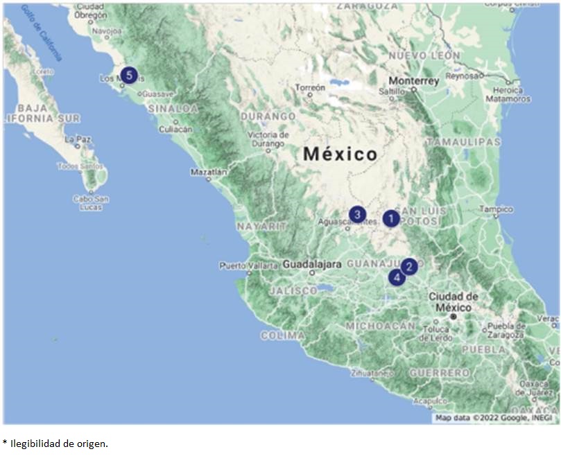
Figure 4 shows the geographical location of the 5 nodes with a higher betweenness value; it stands out for its totally different location that corresponds to El Sufragio, which gives access to the following cities: Guaymas, Hermosillo, Tijuana, Mexicali and Nogales in the north of Mexico; the remaining nodes (San Luis Potosi, Loreto, Salinas, Ing. Buchanan and Celaya) are in the central region of Mexico.
Closeness centrality
To present the results, the same method used for the betweenness was followed; in this case only the probability function in log-log scale is shown; from the value of the correlation coefficient, we accept the hypothesis that the exponential probability distribution adequately adjusts the data (Figure 5).
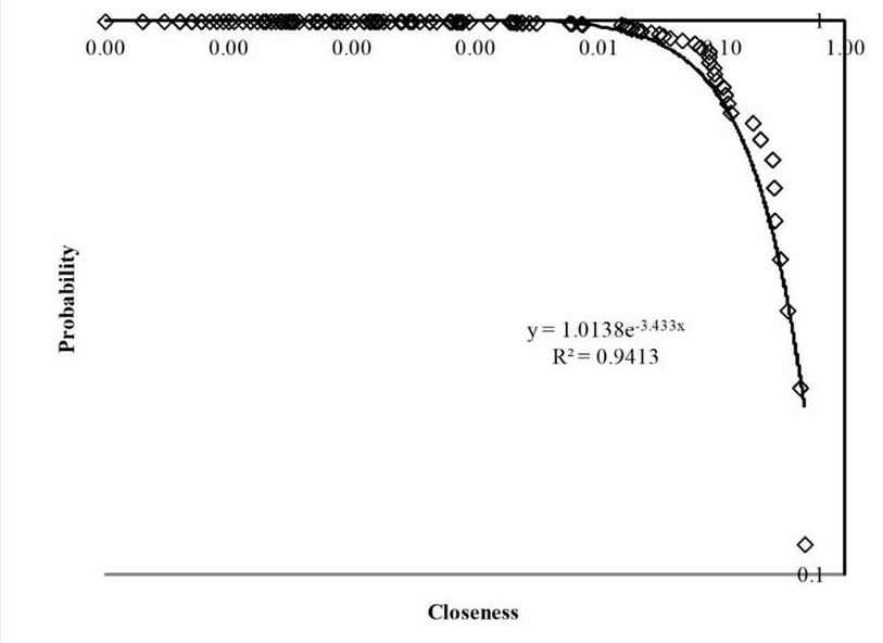
Figure 6 shows the geographical location of the 5 nodes with the highest value of closeness centrality in orange. These nodes are the ones that are closest to any other in the network. Again, Celaya and San Luis Potosí appear in the set of nodes with the greatest closeness centrality value.

Robustness analysis
Method and results
The behavior of the Mexican rail network was analyzed considering random failures and targeted attacks. To remove the nodes, two criteria were followed: for the random failures, a sample of 10 network nodes was generated, later the nodes were removed one by one, after a node was removed the diameter of the largest component, the number of components and the average path length were recorded; finally, the probability distribution of betweenness was plotted.
For directed attacks, the criterion for selecting and removing a node was based on its betweenness value, once the node of the network was eliminated, the betweenness, the diameter, the number of components and the average path length were recalculated; This will show the effect of losing those nodes that control the shortest routes (Iyer et al., 2013; Kuang et al., 2015; Rueda et al., 2017).
The behavior of the diameter of the network is shown in Figure 7. For the case in which the failure is of a random event (grey), the diameter of the network goes from 63 (original value) to 56 after the third node is eliminated; the diameter changes to 54 after the fourth node is removed, then the diameter remains unchanged until the node 10 is eliminated.

The Mexican rail network shows a high sensitivity when the failure occurs in the node with the highest betweenness value (black): when removing the first node, the value of the diameter goes from 63 (original) to 67; when the second node is eliminated, the value of the diameter is 105, by eliminating the third node with the greater value of intermediation the diameter decreases to 96, this is due to the fragmentation of the original network in two subnetworks without communication between them.
Figure 8 shows the number of components for random failures and for the case of directed attack. It is appreciated that the number of components grows faster for the targeted attack scenario. The number of components is 7 after 10 random failures (3.25 % of total); however, when the attack is directed, after eliminating the tenth node the number of components is 14.

When the failures are random, the average path length is 20.223 with a standard deviation of 1.322, which gives a coefficient of variation of C2 R = 0.065; however, in the case of the directed attack, the average path length is 17.68, with a standard deviation of 9.29, which gives a coefficient of variation value C2 D = 0.52 (Figure 9). From the values of the coefficient of variation obtained, it can be said that the average path length has less variability when failures are random than when there are targeted attacks. Finally, we must highlight the increase in the average path length when the 2nd node is disabled due to a directed attack, (Figure 9).

In the case of the betweenness distribution, it can be seen in Figure 10 that as the nodes randomly fail, the probability distribution presents minor change, this can be corroborated in Table 4 by means of the coefficient of variation of the betweenness which shows a difference of 7.23 % between the original value and the value when the fourth failure occurs.

Table 4 Statistics of betweenness after random failures. The results of deleting nodes 1 to 4 are shown
| Scenario | Original | 1 | 2 | 3 | 4 |
|---|---|---|---|---|---|
| Average betweenness | 0.0806 | 0.08721 | 0.0958 | 0.0965 | 0.0984 |
| Standard Deviation | 0.0845 | 0.08353 | 0.0918 | 0.0935 | 0.0962 |
| Coefficient of Variación | 1.048 | 0.957 | 0.958 | 0.968 | 0.977 |
In comparison, when a targeted failure is in course, it can be seen in Figure 11 that as the failures of the nodes are presented, the control of the shorter routes is mediated by a smaller number of nodes; when observing the change in the coefficient of variation it was found that the difference of the original value with respect to the value when the Loreto node fails is 0.94 %; It should be noted that when the Irapuato fails, the rail network breaks down into two disconnected networks and when Guadalajara fails, the network breaks down into 4 disconnected networks (Table 5), the integrity of the network is quickly affected.

Table 5 Statistics of betweenness after malicious attacks. *System with 2 disconnected networks. **System with 4 disconnected networks
| Scenario | Original | San Luis Potosí | Loreto | Irapuato* | Guadalajara** |
|---|---|---|---|---|---|
| Average betweenness | 0.0806 | 0.09065 | 0.146 | 0.0554 | 0.0184 |
| Standard Deviation | 0.0846 | 0.1031 | 0.152 | 0.0567 | 0.0153 |
| Coefficient of Variación | 1.05 | 1.137 | 1.04 | 1.023 | 0.829 |
Conclusions and future work
The results show that the Mexican rail network shares characteristics with other rail networks in the world. It is noted that the average path length and the diameter of the network are smaller than the networks of Switzerland and Europe. Regarding the topology of the network, the conclusions are:
1. In the Mexican rail network, the degree of the nodes (k) follows an exponential probability distribution; this feature is shared with other transportation systems previously analyzed. The exponential probability distribution reflects the physical limitations of real transport systems.
2. According to the betweenness centrality, San Luis Potosi, Loreto, Salinas, Ing. Buchanan, Celaya and El Sufragio, control 19 % of the shortest routes in the networks. Sufragio is the station that controls the access to the following cities: Guaymas, Hermosillo, Tijuana, Mexicali and Nogales.
From the robustness analysis we concluded that:
3. When the failure is directed to nodes with the highest betweenness value, the network fragments into isolated components faster than when there is a random failure.
4. When there are random failures, the probability distribution of the betweenness centrality maintains almost the same location and the control of the shortest routes is maintained by the same nodes, but nevertheless, when the nodes with the highest betweenness fail, the network is overly sensitive.
The results obtained in this research allow to understand the role of the nodes in the structure of the railway network. A manager now knows which nodes are crucial in connectivity and their influence, for example, on the shortest routes.
The structure must be studied further to determine improvements in the system. It is also necessary to conduct an analysis on the effect that the project of the new passenger train will have on the southeast of Mexico.

