


 nueva página del texto (beta)
 Inglés (pdf)
 Artículo en XML
 Referencias del artículo
 Enviar artículo por email
 Citado por SciELO
  Similares en
SciELO
Similares en
SciELO 
 Permalink
Introduction
Mexico is affected by different hazards. One of the most important is the wind hazard, which annually causes great losses due to damage to the infrastructure (Lima et al., 2019; Murià et al., 2018). In fact, there are important databases and records of synoptic winds and various extreme wind events that have affected different areas of Mexico. Based on this, the design of regular structures in Mexico is carried out following the recommendations of the Chapter on The Federal Electricity Comission wind design manual (CFE, 2020). This Chapter has taken into consideration the progress of international standars as the Australian-New Zealand code (AS/NZS (2005) and the Eurocode (2005).
Despite the great effort made to improve the standards for wind design around the world, there are a lot of variables beyond the current guidelines, so it has been necessary to assess these situations with the support of experimental or numerical simulation techniques. Therefore, in Mexico, support was always sought from laboratories of other countries to provide an engineering solution. It is noteworthy that since 1966 internal works for local projects (Sotelo, 1968) were performed in a wind tunnel with 1.20 m height, 0.80 m width and 2.40 m length, where the maximum wind speed was approximately 40 m/s, but due to its geometric characteristics it was very difficult to reproduce artificially the accelerated growth of an atmospheric boundary layer.
According to the National Center for Disaster Prevention (CENAPRED) in Mexico, until 2016 hydro-meteorological phenomena accounted for about 86 % on average of socioeconomic impact of disasters in the last two decades (CENAPRED, 2017). In addition to this, one of the most recent disasters due to a hurricane in Mexico was in Baja California Sur in 2014 due to hurricane Odile, where economic losses were registered about 1.655 million dollars due to the collapse of structures, the interruption of services and loss of contents (Murià et al., 2014), which showed the urgent need to improve and develop experimental wind engineering research in Mexico.
Fortunately, through the efforts of several institutions, companies and universities, with the Institute of Engineering of the UNAM (IIUNAM) as the leader, to improve and promote Mexican Wind Engineering research, in February 2015 a new Boundary Layer Wind Tunnel (BLWT) facility for building environment and structural wind-loading simulations has finally been launched.
For proper operation of the wind tunnel a calibration protocol was proposed, and it should consist of four principal stages. On the first stage the main objective was to represent adequately the lower part of the natural boundary layer by means of different turbulence systems as described in the literature and to achieve this, it was previously necessary to test the performance of the empty wind tunnel. Once this was achieved, the second objective was to compare pressure coefficients of low-rise buildings with free databases and results published in the literature to assure compliance with full-scale measurements, laboratory results and international coding. The third and fourth stages consist of developing tests by the force-balance technique, section and aeroelastic models, respectively, which are out the scope of this work. This paper focuses on the first two stages.
On the first section of this paper a brief description of the new facility at the university is described as well as some of its intrinsic flow characteristics. In the second section the process to perform a boundary layer or surface layer simulation associated to a terrain roughness as well as some of the achieved results desired is fully described. In the third section of the paper, an application of the previous section is used in order to validate building testing. The results in terms of pressure coefficients are compared against those achieved by other wind tunnel facilities. Finally, the conclusions and recommendations are presented at the end of the document.
The boundary layer wind tunnel at UNAM
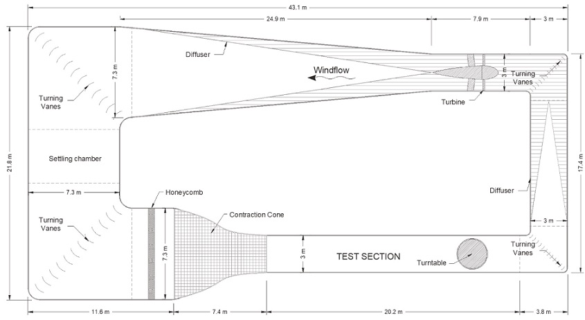
The first design (Figure 1) of the airline of the BLWT was completed in 2005 by personnel of the IIUNAM (Gómez et al., 2011) and then optimized in 2006 by AIOLOS, a Canadian company expert in the design of wind tunnels. Due to this optimization, changes in the geometry at some zones of the original design were modified. One of the most important changes consisted in the addition of a second test section to study aeroelastic and section models of bridges and other structures which test requires a bigger test section.
Geometry of the wind tunnel
The new low-speed boundary layer wind tunnel consists of a closed circuit of simple return with two main testing sections, as shown in Figure 2.

Figure 2 New BLWT of the UNAM: a) plan view, b) lateral view section A-A’, and c) lateral view section B-B’
The BLWT has an overall length of 38.3 m and a width of 14.8 m. It has four main modules. The main function of modules 1 and 3 is to perform structural wind loading tests over the turntables (TTs) located at test section 2, while modules 2 and 4 are mainly used to divert and direct the wind flow. Module 1 has a length of 21 m, with a nearly square section (width and height) about 4 m. While section 2 has also a length of 21 m, a width of 3 m and an adjustable roof from 2 m to 2.4 m height that allows to achieve the zero-pressure gradient at the test section 2.
The fan module (Figure 3) is composed of the fan and its motor that is controlled by a compact Siemens variable-frequency drive (VFD), and the diffusers. The fan diameter is about 3 m and is driven by a low voltage engine, the impeller has 12 blades with a 12° blade pitch which can drive a volume flow rate about 169 m3/s. The VFD is located at the control center and works on a range from 6 to 600 RPM.

The turning vanes, which are used to divert and direct the flow, are made of aluminum, and have a design similar to a quarter circle perimeter with a radius of 0.35 m, a normal straight line of 0.57 m and 0.004 m thick. On module 2, there are 31 turning vanes of 4 m height at each corner, stiffened at a third of their height, and in the other side, on module 4, there are 22 turning vanes of 2.5 m height near the fan module and 22 turning vanes of 2.2 m height near test section 2, both stiffened at mid-height. These elements are beveled at 45°, even the stiffeners are beveled to make them more aerodynamic.
The settling chamber is composed by the heat exchanger, the honeycomb and two screens, followed by the contraction cone. The contraction cone is wooden-made and the honeycomb is structured by 10 rectangular module panels of 1.20 width x 2.40 m height.
The TTs are wooden-made and can be activated by a system that controls the rotation of the tables. This system can also be operated semi-manually from touch screens, located in the control center, or digitally with a software programed on LabVIEW from the main computer at the control center. More than 700 wind incidence angles can be studied, since TTs can rotate every 0.5° in a range from -179° to 179°.
Performance of the wind tunnel
First, it was necessary to identify the characteristics of the wind flow in modules 1 and 3. The purpose of these measurements was to estimate the expected mean wind speed, gradient height and turbulence intensity in different locations of the test section and to associate these values with the RPM of the turbine with the empty wind tunnel. In module 3, a total of 7 stations to carry out the flow measurements were selected, as shown in Figure 4.
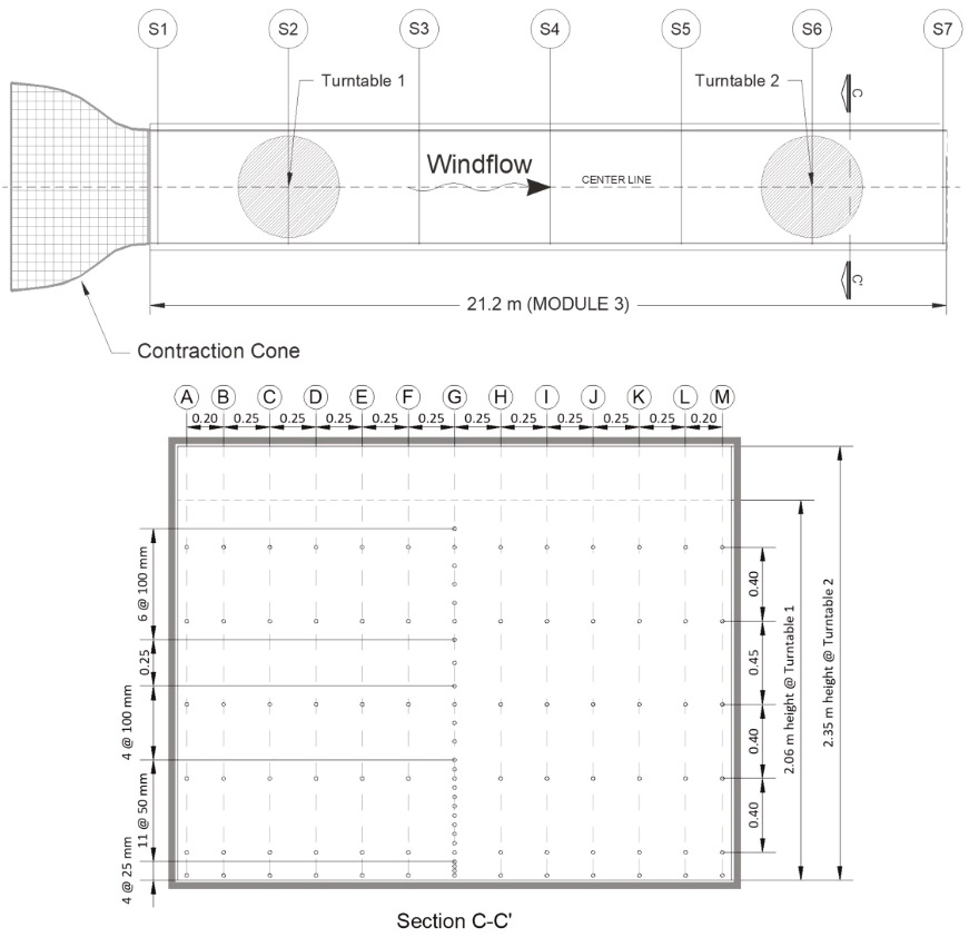
The velocity and its turbulent fluctuations were measured in the longitudinal direction by using a single channel Dantec Dynamic’s MiniCTA 54T42 anemometry system, which included a 55H20 short single-sensor probe with a 55P11 miniature wire probe. The data acquisition was made with a NI cDAQ-9171 card controlled by a personal computer. A calibration of the MiniCTA 54T42 anemometry system was carried out by using a Pitot-static tube to define the velocity reference. The Pitot-static tube and the 55H20 short single-sensor probe were located at the center line of TT2, at mid-height (Station S6). A total of 10 velocity references were measured with the Pitot-static tube, each one associated with a rotational speed of the turbine within the range from 105 to 600 RPM. During the measurements of the velocity reference, temperature was registered with a digital thermometer connected to a probe located close to the Pitot-static tube. The velocity references were used to relate the voltage registered with the 55H20 short single-sensor probe by using the Dantec Dynamics Streamware Basic© application software. Temperature corrections were included in the calibration process.
Once the hot wire anemometer (HWA) was calibrated, flow measurements were made at Stations 2 and 6 (TTs) according to the distribution shown in Figure 4b. For the rest of the Stations, the flow measurements were recorded only at the G axis.
A sketch of the normalized profiles of mean wind speed and turbulence intensity, as well as the gradient height along the main test section of the wind tunnel are presented in Figure 5. To better compare the profiles, a normalized length of the main test section (starting at the exit of the contraction cone and ending at the entrance of Corner 1) was used in the horizontal axis of Figure 5. The values shown in this figure correspond to the G axis of each Station (see Figure 4a). In Figure 5, the solid lines correspond to the mean velocity profile, while the triangles correspond to the turbulence intensity. It can be observed in Figure 5 that there is an increase in turbulence from stations S2 to S6, due to friction of the floor of the tunnel that is accumulating upstream from one point to another. It can also be noted that the gradient height remains constant from Stations S5 to S6 due to the change of floor’s roughness from one point to another (from rubber to smooth wood). Table 1 summarizes the values of the mean wind speed and turbulence intensity at gradient height from Figure 5.
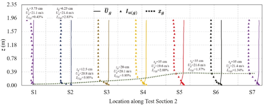
Figure 5 Gradient height along the center line (G axis) of test section 2. The normalized profiles of mean wind speed and turbulence intensity are schematically shown for reference
Table 1 Summary of gradient height, gradient velocities and turbulence intensities at gradient height (see Figures 4 and 5)
| Station | zg (cm) |
|
I(u(g)) (%) |
| S1 | 3.75 | 21.08 | 0.43 |
| S2 | 6.25 | 21.42 | 2.83 |
| S3 | 12.50 | 20.79 | 3.95 |
| S4 | 20.00 | 20.13 | 3.95 |
| S5 | 35.00 | 19.60 | 2.88 |
| S6 | 35.00 | 21.57 | 1.37 |
| S7 | 35.00 | 21.41 | 1.34 |
The data of experimental velocities for the empty wind tunnel condition were adjusted by using the log-law (Equation 1) and the power law (Equation 2) by means of linear regressions:
Where:
u *= |
represents the friction velocity |
κ = |
the Von Karman constant defided as 4.0 |
z = |
the height |
d = |
the zero-plane displacement |
z0 = |
the roughness length and |
α = |
the index parameter for the power-law |
The parameters found from the fitting were at turntable 1 (TT1), u * =0.77 m/s, z 0=9.70x10⁻⁶ m and α=0.05, while at turntable 2 (TT2), the fitting gave u * =0.72 m/s, z 0=9.70x10⁻⁶ and α =0.11.
As expressed by Wittwer and Möller (2000) the evaluation of capabilities, scopes and other characteristics of many wind tunnels is usually presented in the literature as a way to compare and validate wind tunnel testing, especially for empty conditions. A comparison of the most important wind tunnel facilities around the globe is summarized in Table 2, where the country, the name of the laboratory, the year in which the facility information was published, the dimensions of the main test section, the maximum wind speed and turbulence intensity achieved on empty conditions are presented.
Table 2 Comparison of some wind tunnels around the world
| Country | Wind tunnel | Year* | Type of Circuit | Main working section | Ux (m/s) | Iux (%) |
| Argentina | UNNE Wind Tunnel (Wittwer & Möller, 2000) | 2000 | Closed | W 2.4 x H 1.8 x L 22.8 m | 27 | 1.0 - 3.0 |
| Australia | WINDTECH Consultants BLWT3 | 1991 | Open | W 3.0 x H 2.0 x L 23.0 m | - | - |
| Belgium | von Karman Institute for Fluid Dynamics L-1B | - | - | W 3.0 x H 2.0 x L 20.0 m | 50 | - |
| Brazil | UFRGS Boundary Layer TV-2 Wind Tunnel (Blessmann, 1982) | 1982 | Closed | W 1.3 x H 0.9 x L 9.32 m | 42 | < 0.5 |
| Canada | The Centre for Building Studies of Concordia University (Stathopoulos, 1984) | 1984 | - | W 1.8 x H 1.8 x L 12.0 m | 14 | - |
| Canada | University of Western Ontario (UWO) BLWT1 | 1965 | Open | W 3.4 x H 2.5 x L 39.0 m | - | - |
| Canada | Rowan Williams Davies & Irwin Inc. (RWDI) | 1972 | - | W 2.4 x H 2.0 x L ¿? m | - | - |
| Canada | UWO BLWT2: Alan Davenport's Group | 1984 | Closed | W 3.4 x H 2.5 x L 39.0 m | - | - |
| Canada | UWO WindEEE Dome | 2011 | Closed | Ø 25.0 x H 3.8 | - | - |
| China | Tongji University TJ-2 Wind Tunnel | - | - | W 3.0 x H 2.5 x L 15.0 m | 18 | - |
| China | Tongji University TJ-3 Wind Tunnel | - | - | W 15.0 x H 2.0 x L 14.0 m | 15 | - |
| China | Southwest Jiaotong University SWJTU-3 | 2008 | - | W 22.5 x H 4.5 x L 36.0 m | 17 | < 1.0 |
| China | Shantou University | - | - | W 3.0 x H 2.0 x L 20.0 m | - | - |
| Denmark | Force Technology BLWT (WT2) | - | Open | W 2.6 x H 1.8-2.3 x L 20.8 m | 24 | - |
| England | Bristol University (Barret, 1972) | 1972 | - | W 2.0 x H 1.0 x L 5.25 m | 18 | - |
| England | BRE Boundary Layer Wind Tunnel (Cook, 1975) | 1975 | Open | W 2.0 x H 1.0 x L 8.0 m | 20 | - |
| England | The City University Wind Tunnel (Skyes, 1977) | 1977 | - | W 3.0 x H 1.5 x L 8.1 m | 26 | - |
| England | Cranfield University BLWT | - | Open | W 2.4 x H 1.2 x L 15.0 m | 16 | < 0.5 |
| England | EnFlo Meteorological Wind Tunnel | - | - | W 3.5 x H 1.5 x L 20.0 m | 3 | - |
| Germany | Ruhr University | - | Open | W 1.8 x H 1.6 x L 9.4 m | - | - |
| Germany | Universität Hamburg (UH) WOTAN BLWT | - | - | W 4.0 x H 2.75-3.25 x L 25.0 m | 20 | - |
| Italy | Politecnico di Milano Civil-Aeronautical Wind Tunnel (Diana et al., 1998) | 1998 | - | W 3.8 x H 3.8 x L 13.8 m | 15 | < 2.0 |
| Italy | Inter-University Research Centre on Building Aerodynamics and Wind Engineering (CRIACIV) | - | - | W 2.42 x H 1.60 x L 10.0 m | 30 | - |
| Japan | Tokyo Polytechnic University (TPU) BLWT | - | Open | W 2.2 x H 1.8 x L 14.0 m | - | - |
| Japan | Research Institute for Applied Mechanics Thermally Stratified Wind Tunnel | 1995 | Open | W 1.5 x H 1.2 x L 13.5 m | - | < 3.0 |
| Japan | 2D Actively Controlled Wind Tunnel | - | - | W 0.18 x H 1.0 x L 3.8 m | - | - |
| Mexico | UNAM BLWT | 2015 | Closed | W 3.0 x H 2.0-2.4 x L 21.0 m | 22 | 1.0 - 4.0 |
| Netherlands | Technische Universiteit Eindhoven (TU/e) Wind Tunnel | 2017 | Closed | W 3.0 x H 2.0 x L 27.0 m | - | - |
| Rumania | Universitatea Tehnică de Construcții din București (UTCB) TASL1-M BLWT (Vladut et al., 2017) | 2013 | Open | W 1.75 x H 1.75 x L 27.0 m | 17 | < 1.0 |
| Singapore | NUS-HDB Wind Tunnel (Balendra et al., 2002) | 2002 | Closed | W 2.85 x H 1.8-2.3 x L 19.0 m | 15 | < 1.0 |
| Spain | Ignacio Da Riva University Institute of Microgravity of the Madrid Polytechnic University (IDR/UPM) Aerodynamic Tunnel ACLA16 | 2009 | Closed | W 2.2 x H 2.2 x L 20.0 m | 35 | - |
| USA | St. Anthony Falls Lab (SAFL) BLWT | 1984 | Closed |
W 1.5 x H 1.7
x L 16.0 m W 2.4 x H 2.4 x L 18.0 m |
45 19 | - |
| USA | Texas Tech University (TTU) / National Wind Institute | - | Closed | W 1.83 x H 1.22 x L 17.68 m | 49 | - |
| USA | TTU Wind Engineering Research Field Laboratory (WERFL) | 1989 | - | - | - | - |
Note: Dimensions of the main test section (W = width; H = height; L = length); *First publication or opening year.
Boundary layer simulation
The mean velocity profile, turbulence intensity as well as spectral measurements are usually considered to evaluate the quality of a wind tunnel to simulate the characteristics of the atmospheric boundary layer (Counihan, 1969, 1973; Cook, 1978b; Irwin, 1981; Cermak, 1995). In this study, two methods were used to simulate the same terrain category, considering full (Counihan, 1975; Farell and Iyengar, 1999) and part-depth simulations (Cook, 1973; Cermak et al., 1995; De Bortoli et al., 2002; Kozmar, 2011).
Full and part-depth simulations
Experimental setup
The full depth simulations were carried out by using the methods established by Counihan (1969, 1973), Standen (1972) and Robins (1979), while the part-depth simulations were carried out by using Irwin’s method (Irwin, 1981) and modifications of it as several authors have done. As a starting point to calibrate and understand the artificial simulation of different terrain categories in the laboratory and so to minimize calibration time for the simulation of an urban-type artificial terrain, a system was designed to generate turbulence, guided by the arrangement and results reported by Balendra et al. (2002) by making some minor modifications to the arrangement, since the NUS-HDB dimensions are similar to those at UNAM’s BLWT. The devices employed to simulate the full/part-depth with Counihan’s and Irwin’s methods are shown in Figure 6.
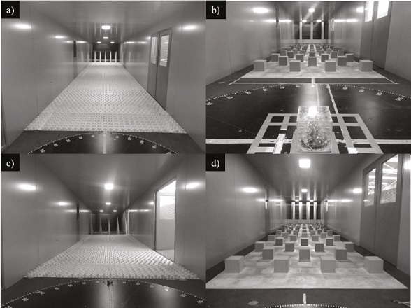
Figure 6 Devices for urban simulation with: a) Counihan’s full-depth simulation, b) Counihan’s part-depth simulation, c) Irwin’s full-depth simulation, d) Irwin’s part-depth simulation
Cubic and prismatic elements were used as roughness elements along the main section of the test (module 3). The dimensions of the roughness elements and the type of arrangement used are summarized in Table 3.
Table 3 Summary of dimensions and arrangement of roughness elements
| Characteristic | Cubic elements | Prismatic elements | Main References | ||
| FDS | PDS | FDS | PDS | ||
| Base x Depth x Height (m) | 0.03 x 0.03 x 0.03 | 0.20 x 0.20 x 0.20 | 0.03 x 0.03 x 0.06 | n/a | Counihan (1969, 1973) |
| Fetch of roughness elements (m) | 13.61 | 12.52 | 0.77 | n/a | Irwin (1981) |
| Distance between centers of elements along the width of the WT* (m) |
0.11 / 0.055 | 0.7 | 0.11 | n/a | Balendra et al. (2002)) |
| Distance between centers of elements
along the length of the WT* (m) |
0.11 / 0.055 | 0.7 | 0.11 | n/a | |
| Type of arrangement | Staggered | ||||
* The minor distance refers to elements on the minor fetch
Two boundary layer depths for the same terrain category were simulated, the
full-depth simulation to replicate the Atmospheric Boundary Layer (ABL) of an
urban terrain has a length scale of 1:410 and based on the recommendations of
Tieleman (Tieleman, 2003) for low-rise
buildings, to simulate the Atmospheric Surface Layer (ASL) the part-depth
simulation an initial model scale factor 1:50 was assumed. To perform the
full-depth simulation with the Counihan’s method (FDC), a castellated barrier, a
fetch of roughness elements and 5 elliptical wedge vortex generators were used,
while, for the part-depth simulation with the Counihan’s method (PDC), a
straight barrier, a set of larger roughness elements and 3 elliptical wedge
vortex generators were truncated as suggested by Kozmar (2011). Further, for the full-depth simulation with the
Irwin’s method (FDI), the castellated barrier, the elliptical vortex generators
and some roughness elements were replaced by 5 triangular spires, while, for the
part-depth simulation with the Irwin’s method (PDI), 4 truncated spires were
used as suggested by several authors (Ham &
Bienkiewicz, 1998; Endo et
al., 2006; Irwin,
2008; Dagnew & Bitsuamlak,
2013). Usually the full-depth tests are carried out at the maximum
speed of the fan to validate the velocity profile in a given site; however,
since in Mexico there are at least two cities with the same density of buildings
(i.e., Monterrey (MTY) and Mexico City (CDMX)) it was proposed to test the same
artificial urban terrain under two different velocities, at the highest speed of
the fan and at a relatively lower speed, respectively. According to the manual
of civil works for wind design (CFE,
2008), the regional wind speed at 10 m associated with a return period of
50 years for Monterrey is
To perform a more consistent simulation, the criterion adapted in this study was that the similarity of the velocity scale should remain the same for both the full-depth and the part-depth simulations, varying length and frequency scales. This should obtain the same wind velocity magnitude at the same reference height for one scale or another in lab. The velocity records during the tests were made at a sampling frequency of 2000 Hz for both the ABL and ASL simulations. For the ASL simulation, a cutoff frequency was applied at 256 Hz.
Results
The records of mean and fluctuating wind speed were registered at the center of the TT2 using the HWA. The records of the full-depth simulations were adjusted considering a gradient height, z ABL= 490 m, while the data of the part-depth simulations were adjusted to the typical atmospheric surface layer height, z ASL= 100 m.
Equations 1 and 2 were employed to estimate the parameters used to characterize the mean wind profile, in most cases, the best fit was obtained with the power-law function when using both the Counihan’s and the Irwin’s method. A summary of the estimated parameters for both full-depth and part-depth simulations is presented in Table 4.
Table 4 Summary of data fitting
| Variable (units) | Full-depth simulations (ABL) | Part-depth simulations (ASL) | |||||||
| FDC(MTY) | FDC(CDMX) | FDI(MTY) | FDI(CDMX) | PDC(MTY) | PDC(CDMX) | PDI(MTY) | PDI(CDMX) | ||
| u* | (m/s) | 1.58 | 1.44 | 1.77 | 1.68 | 1.57 | 1.3 | 1.44 | 1.08 |
| z0 | (m) | 0.0071 | 0.0064 | 0.0121 | 0.0131 | 0.0358 | 0.0326 | 0.0393 | 0.0369 |
| d | (m) | 0 | 0 | 0 | 0 | 0 | 0 | 0 | 0 |
| α | 0.29 | 0.28 | 0.35 | 0.37 | 0.31 | 0.28 | 0.26 | 0.26 | |
| Lxu | (m) | 48 | 64 | 48 | 67 | 63 | 54 | 58 | 50 |
| S | 462 | 318 | 448 | 280 | 4.4 | 5.7 | 4.4 | 5.4 | |
Figures 7 and 8 show the mean velocity profiles and turbulence intensities, respectively, for the simulations considered. In these figures, hollow markers are used to represent the data from the full-depth simulations and filled markers to represent the data from the part-depth simulations. It is observed in Figure 7 that all the mean velocity profiles for the part-depth simulations agree well with the full-depth data. It is observed in Figure 8 that there are some differences on the longitudinal turbulence intensity of the part-depth simulation that should be further investigated. In Figure 8, to compare the experimental results, the equations proposed by Walshe (1973), Holmes (2007) and ESDU (1974, 1985) to describe the turbulence intensity variation with height were employed. When comparing the experimental data with the empirical expressions it can be noted that full-depth turbulence intensities agree well with the empirical equations up to a range from 200-400 m height, after those levels, lower turbulence intensities were registered as reported by Farell & Iyengar (1999). The turbulence intensities for the part-depth simulation seem to agree well with Walshe’s expression. According to Counihan (1975) and Balendra et al. (2002), for urban environments up to 30 m height, turbulence intensity should vary in the range of 20-35 %. Based on these observations, the experimental data agree relatively well with Walshe’s expression from 30 to 50 m height, where turbulence intensities vary from 19 to 28 %, similar to the values reported by Hölscher & Niemann (1998).

Figure 7 Full-scale longitudinal velocity distribution for all simulations. Hollow markers = ABL simulations (1:410) and filled markers = ASL simulations (1:50) for low and high velocities (Monterrey and CDMX respectively) for the same roughness (urban terrain). Inside, a close-up of the first 100 m of the profile is shown
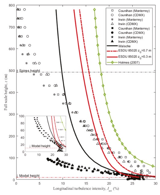
Figure 8 Full-scale longitudinal turbulence intensity for all simulations. Hollow markers = ABL simulations (FDC and FDI) and filled markers = ASL simulations (PDC and PDI) for low and high velocities (Monterrey and CDMX respectively) for the same roughness (urban terrain). Inside, a close-up of the first 100 m of the profile is shown
Figure 9 shows the experimental spectral data fitted with the von Karman’s and Kaimal’s spectra at model height for the FDC and FDI simulations, respectively. It is observed good agreement between the experimental data and the theoretical expressions. The integral length scales of turbulence (L x u ) were obtained by fitting the measured data to the von Karman’s and Kaimal’s spectra, given by the following equations, respectively,
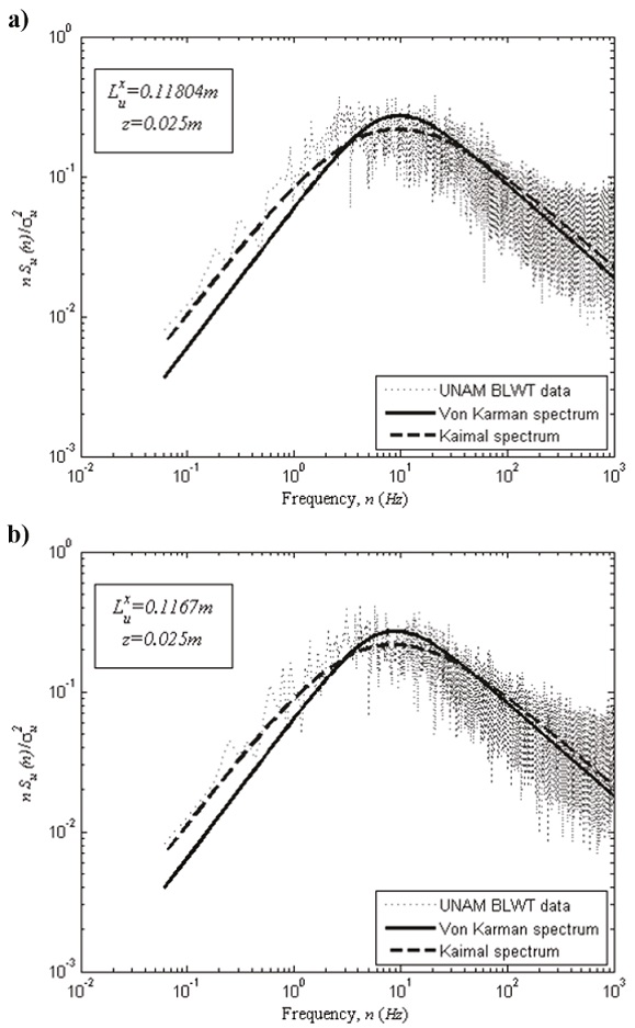
Figure 9 Spectrum of turbulence in the along-wind direction at model height for urban ABL with a) FDC and b) FDI
where n is the frequency, S u (n) is the power spectrum of the longitudinal velocity, f z is the reduced frequency, defined as n z=U, σu is the standard deviation of the fluctuating velocity component in the streamwise direction while f L is the non-dimensional frequency (n L x u /U).
Figure 10 shows a comparison of the full-scale longitudinal integral length scales for the FDC, PDC, FDI and PDI simulations. In Figure 10, the integral length scales calculated according to Walshe (1973) and ESDU (1974, 1985) are also included. It is observed in Figure 10 good agreement between the experimental and theoretical expressions, mainly for FDC simulations.

Figure 10 Full-scale longitudinal integral length scales for all simulations (FDC = full-depth with Counihan’s method; FDI = full-depth with Irwin’s method; PDC = partial-depth with Counihan’s method; PDI = partial-depth with Irwin’s method; ESDU = Engineering Sciences Data Unit; Walsche’s method (1973)). Inside, a close-up of the first 100 m of the profile is shown
The turbulent length scales were used to calculate, in a deterministic way, the model scale factor, S (Equation 6) (Cook, 1978a) to compare with the model scale factor initially proposed:
where z is the corresponding measured height, d is the zero-plane displacement, L x u is the integral length scale in the longitudinal wind direction and z 0 is the roughness length of the terrain. The model scale factors calculated with Equation 5 are summarized in Table 4. For the full-depth simulation, the model scale factor calculated with Equation 5 are in the interval 280 < L x u < 462, and those for the part-depth simulation are 46 < L x u < 59. In general, the scale factors initially proposed are within the estimated intervals.
Testing of pressure models
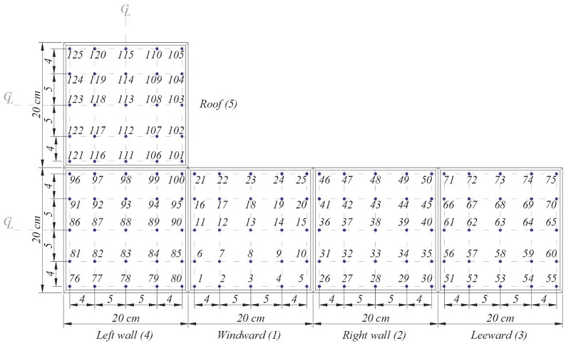
To calibrate the tests of rigid models, a cubic model with a length scale of 1:50 was designed. This type of configuration has been widely studied around the world (Richards et al., 2001, 2007; Hunt, 1982; Castro & Robins, 1977; Tokyo Polytechnic University, 2007). Moreover, an effective blocking ratio < 5 % (Tieleman, 2003) was considered and it was assumed a prototype with 10 m height, thus, it was determined that the model height should be h m=0.20 m. The cube was placed on the TT2 of the main test section, and due to the symmetry of the model, it was considered enough to study only 21 wind directions, in a range θ=-90° ~ 90°. The prototype Jensen number to relate the roughness length of the terrain and the height of the structure (Jensen, 1958) was Je (P)=5. The model was built with 0.004 m thick acrylic plates to guarantee its stiffness and to be able to observe the plastic tubes inside the model from the outside. To select the location of each of the pressure taps, the following was considered: 1) the distribution of pressure taps used by other authors for the same type of models, 2) the distribution of pressure coefficient contours from experimental and numerical models (CFD); and 3) the number of pressure transducers available at the time the tests were performed. With this, 125 pressure sensors were determined to be adequate for the model as shown in Figure 11.
The acquisition system to get the pressure time-histories consists of series of urethane plastic tubes (Scanivalve’s URTH-040 plastic tubing) added to the model surfaces and linked to miniature pressure scanners (Scanivalve’s ZOC22b). The miniature pressure scanners transmit the information to an A/D converter (Scanivalve’s DSM4000).
The sampling frequency for the model was 256 Hz, and the sampling time was 45 s, which corresponds to a sampling frequency of 9.6 Hz and 10 min period at full scale. Based on the above, a total of 11,520 samples/tap was obtained. Figure 12 shows the mean pressure coefficients at different reference lines around the model.

Figure 12 Comparisons of external pressure coefficients over: a) the center-vertical line, b) the center-horizontal line and c) the cross-vertical line in the along-wind direction (θ=0o)
It is observed in Figure 12 that the experimental results from the IIUNAM (i.e., present study) are comparable with those reported by Richards et al. (2001, 2007) (i.e., the full-scale model) and the TPU (2007). Important differences are observed in Figure 12 between several authors (Baines, 1963; Castro and Robins, 1977; Hunt, 1982; Hölscher & Niemann, 1998; Richards et al., 2007; TPU, 2007; CFE, 2008; NTC-DV, 2017) for the same model. These variations may be due to several reasons, such as the artificial turbulence system, equipment, and sampling frequency, taps length, air temperature or turbulence intensities, as reported by Hölscher & Niemann (1998). In Figure 12a it was observed that the maximum differences in the windward wall between all the simulations is about 30 %, while in the areas of negative pressure, i.e., the roof and leeward zones, the observed maximum differences are about 40-60 %. Similar high differences for the pressure coefficients over the distinct model zones and between different facilities simulations were highlighted by Hölscher & Niemann (1998). Likewise, between the TPU database (2007) and the IIUNAM, the observed differences on the windward wall are less than 5 %, while for the roof and the leeward wall, the observed differences are less than 10 %. Also, in Figure 12b general variations between different authors are observed around 40 % and variations close to 5 % in the windward zone, and 15 % in the negative pressure zones between the TPU and the IIUNAM. Similarly, in Figure 12c there are also general variations between different authors around 40 % and variations around 20 % in the walls and the roof, between the TPU and the IIUNAM. In general, the estimated pressure coefficient values by the IIUNAM seem to agree well with the Mexican manual (CFE, 2008) and the Mexican standard (NTC-DV, 2017), except on the roof, where the NTC-DV (2017) indicates lower values.
Based on the comparisons made with the cube model, it was considered that the results obtained for the rest of the models were adequate, since the conditions of the tests and the handling of pressure and pressure coefficient records were applied to the same way as in the cube model. It is considered that, in order to improve the experimental simulations, it would be necessary to study reattachment lengths for roof-separation bubbles since these mechanisms may cause large uplifting loads on the roofs of LRBs (Tieleman, 2006; Akon & Kopp, 2016, 2018). However, this is only possible with a Particle Image Velocimetry (PIV) technique that is not yet available in the new IIUNAM BLWT.
Conclusions
A description of the characteristics and calibration of the boundary layer wind tunnel at IIUNAM was presented. The flow characteristics with the empty wind tunnel, the results of the part-depth and full-depth simulation and the distribution of the mean pressure coefficients on a cubic model were presented. More details about the findings during the stage of calibration are:
The tests with the empty wind tunnel show that the average and fluctuating characteristics of the wind flow are similar to those obtained in other laboratories, especially those reported by Wittwer & Möller (2000), Blessmann (1982) and Balendra et al. (2002).
While using the same velocity scale for different lab length scales, it was observed that the Counihan’s method for artificial full-depth simulation presented better agreement with the atmospheric data, while for the part-depth simulation, the Irwin’s method presented better results. Further investigation is required to determine which passive turbulence method is better for certain type of simulations.
The quality of the turbulence profiles needs to be improved for future projects. To improve both turbulence intensity profiles and integral length scale profiles, especially for the partial depth simulation, devices such as a turbulence grids, could be implemented as observed in studies conducted by Stathopoulos et al. (2008), Biqing et al. (2011) and Aly (2013).
The comparison between the estimated power spectral density function with Kaimal’s and von Karman’s empirical expressions showed good agreement since the experimental data presents the same slope (-5/3) in the inertial subrange of the Kolmogorov’s energy cascade.
The pressure coefficients obtained from the model of a cube agree well with those reported in the specialized literature, especially with those reported by the aerodynamic database of the TPU (2007), where differences close to 5 % were obtained in the windward zone and around a 15 % in the flow detachment zones, i.e., the roof and the leeward wall.
It was observed that, in the light of the results, the pressure coefficients available in the current Mexican regulations may need to be updated to perform better structural designs against wind effects but further analyses are still required to assess this statement.
Finally, although other types of tests are under calibration, it is considered that the new boundary layer wind tunnel of the UNAM can be used to test different type of structures with confidence and contribute to the development of the Mexican wind engineering.
Nomenclature
ABL |
Atmoshperic Boundary Layer |
ASL |
Atmoshperic Surface Layer |
α |
Power law or wind shear exponent that varies depending upon the stability of the atmosphere or the terrain category |
BLWT |
Boundary Layer Wind Tunnel |
CENAPRED |
National Center for Disaster Prevention |
d |
Zero plane displacement, m |
ESDU |
Engineering Sciences Data Unit |
FDC |
Full-depth with the Counihan’s method |
FDI |
Full-depth simulation with the Irwin’s method |
H |
Building height, m |
HWA |
Hot wire anemometer |
IIUNAM |
Institute of Engineering of the UNAM |
IUx |
Longitudinal turbulence intensity, % |
Je(P) |
Jensen number of the prototype |
k |
von Karman’s constant (≈0.40) |
L |
Building length, m |
LRB(s) |
Low Rise-Building(s) |
Lxu |
Integral length scales of turbulence |
NUS-HDB |
National University of Singapore funded by Housing Development Board |
PDC |
Part-depth simulation with the Counihan’s method |
PDI |
Part-depth simulation with the Irwin’s method |
θ |
Wind direction |
RPM |
Revolutions per minute |
S |
Model scale factor |
TPU |
Tokyo Polytechnic University |
TT1, TT2 |
First or second turntable |
u*,u*ABL* |
ABL friction velocity, m/s |
Ux, U(z) |
Mean longitudinal velocity at a distance above ground, m/s |
Ug |
Gradient velocity, m/s |
Uref |
Mean velocity at reference height, m/s |
UNAM |
National Autonomous University of Mexico |
VFD |
Variable-frequency drive |
W |
Building width, m |
z |
Vertical coordinate, m |
z0 |
Roughness length, m |
zABL |
ASL height, m |
zg, zABL |
Gradient height or ABL height, m |

