


 nueva página del texto (beta)
 Inglés (pdf)
 Artículo en XML
 Referencias del artículo
 Enviar artículo por email
 Citado por SciELO
  Similares en
SciELO
Similares en
SciELO 
 Permalink
Introduction
Ambient seismic noise has been widely used to study the seismic response of soft soil deposits using the horizontal-to-vertical spectral ratio (HVSR) (Nakamura, 1989; Field et al., 1990; Bard, 1999). The main application of HVSR is seismic microzoning for cities mainly located in sedimentary basins (Lermo & Chávez, 1994a b; Field & Jacob, 1995). The seismic noise nature could be classified as that produced by natural activities at frequencies less than 1 Hz (Oceanic, Meteorological) and frequencies higher than 1 Hz produced by human activities (Bonnefoy et al., 2006). In a broad frequency band, seismic noise is mainly formed by surface waves (e.g., Schuster, 2014). The extraction of the dispersive properties of these waves then allows determining the structure of S wave velocity of subsoil. The use of seismic noise has advantages over seismic methods using active sources. For example, studies are appropriated out in urban environments, and greater depth of penetration can be achieved through low-frequency seismic noise.
The use of station arrays has allowed the noise to be composed predominantly of surface waves. There are different microtremor analysis methodologies (Socco et al., 2010) that seek to reliably determine the phase velocity dispersion curve of the fundamental mode of Rayleigh waves. The emphasis is on the characterization of the structure of the subsoil to have recognition advantages beyond what geotechnical techniques can provide (Okada, 2006). The most widely used and developed method, with regular and irregular arrays, is the spatial autocorrelation SPAC method (Wathelet et al., 2008) proposed by Aki (1957) . The method assumes that the seismic noise field is a stochastic stationary process in time and space. Under this assumption, Chávez et al. (2005) show that the dispersion characteristics of the surface waves contained in the noise can be extracted, operating only a couple of stations. In linear arrays, and similar to the active MASW method (Park et al., 1999), the microtremor refraction method, ReMi (Louie 2001), offers a practical alternative to exploring the subsoil in the first tens of meters.
Among seismic noise methods, one method that can create a 3D representation of the structure of the subsoil (without the need for a source for mechanical wave generation) is ambient seismic noise interferometry tomography (ANT). Seismic interferometry (SI) makes use of cross-correlation of noise between pair stations to extract the so-called impulse response or Empirical Green Function (EGF) (e.g., Campillo & Paul, 2003; Draganov et al., 2007; Schuster, 2014). The EGF is primarily formed by surface waves whose dispersion characteristics can be measured over a broad range of frequencies (Shapiro, 2004; Gouedard et al., 2008). A summary of the historical background and a variety of applications in various fields of science can be found within, e.g., Schuster (2014), Larose et al. (2015).
In this study, we applied the ANT method to characterize the subsoil velocity structure at a site where a school building was currently built. The problem of the site is there are cavities or lava tubes due to basaltic spills from the eruption of the Xitle volcano, whose lava formed the so-called zone of the pedregal. Our objective is to explore subsoil discontinuities that can constitute a risk for building foundation. Because the method assumes the noise field contains surface waves that propagate in a stratified medium, in a first step, we explored the presence of a soft soil deposit employing the HVSR method in 16 measurements of ambient noise. Subsequently, we developed seismic noise tomography images from cross-correlations of the ambient noise recorded in a rectangular array with 48 vertical geophones. Ultimately, we present a 3D model of the shear wave velocity that we derive from the inversion of dispersion curves constructed from tomography images.
Study zone
The study site is located in the so-called Engineering Annex, which consists of a set of buildings of the School of Engineering at National Autonomous University of Mexico (UNAM). These buildings are constructed on a mixed base of soil and basalt rock characteristic of the university campus. The site is classified as a firm zone according to the geotechnical zoning of Mexico City (Lermo & Chávez, 1994a). In the area, the basaltic flows of the Xitle volcano stand out, whose eruption begins in a strombolian manner with a moderately explosive eruptive style (Siebe, 2009; Cervantes & Wallace, 2003). The successive eruptive stages resulted in lava flows that interspersed and overlapped with each other. These lavas descended at distances of approximately 12 km until reaching the southern plains of the valley of Mexico, where they covered the areas that currently occupy the urban developments of Tlalpan, Coyoacán, and Álvaro Obregón municipalities (Siebe, 2009). Because of the low viscosity and elevated temperature of the lava (>1000° C), these were solidified, leaving cavities or tunnels that are still preserved, as an example, the old name of Tlalpan, which in the nineteenth century was known as San Agustin de las Cuevas.
Figure 1 shows the location of the study site, which is limited by the parking areas of the faculty of accounting and administration (western side) and engineering annex (eastern side). A road circuit is located to the south, and to the north, the building J, whose basement is irregularly shaped because it was adapted to the pre-existing morphology. At the site, we performed 16 measurements of ambient noise using Guralp system 6TD broadband triaxial seismographs. Next, we installed an array of 48 vertical geophones of 4.5 Hz with separations of 3 and 4 m to surround an approximate area of 36 x 56 m2. The ambient seismic noise for tomography imaging was recorded for 60 min using four EX12 seismographs of Seistronix Instrument.
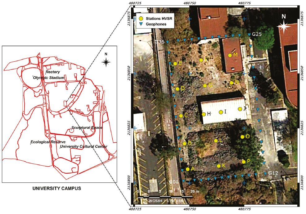
Figure 1: Study site. The blue triangles show the position of the 4.5 Hz vertical geophones. The vertices of the array are indicated with the nomenclature denoting the geophone number G01, G12, G25, and G36. The yellow circles denoted by the letters A to P indicate the points where the HVSR was applied
The horizontal-to-vertical spectral ratio (HVSR)
The HVSR, or commonly referred to as the Nakamura method (Nakamura, 1989), is used to evaluate the site effect, i.e., the relative amplification of the subsoil due to the presence of a soft soil layer and the frequency at which this amplification occurs. The method makes use of ambient seismic noise by assuming the wave field is predominantly formed by surface waves (Bonnefoy et al., 2006). If the layer is present, the spectral ratio of the average Fourier amplitude spectra of horizontal components, among the amplitude spectrum of vertical component, provides the seismic response of the soft layer. The frequency where the maximum response appears is called the fundamental frequency of vibration of the soil layer (f0). The Nakamura method represents a suitable approach to amplification due to S-wave resonance (Lermo & Chávez, 1994b). Therefore, it is possible to approximate the thickness of the soft soil layer (if it exists) by the formulation f0=β/4H.
Where:
f0 = fundamental frequency
β = shear-wave velocity and
H = layer thickness
In the assessment of the HVSR, we used 30 min of ambient noise recording to obtain the average spectral ratio result of windows of 40s duration with an overlap of 50 %. In this estimate, the spectra were smoothed by a Konno-Ohmachi window (Konno & Ohmachi, 1998) with a smoothening fraction of 20 %.
Figure 2 shows the average HVSR curves of the 16 measurement points shown in Figure 1. Except for points P and L, the results show well-defined spectral ratios with an average relative amplification between 2 and 3. These ratios convincingly indicate the distribution of unconsolidated materials overlaying a more competent layer (interpretation criterion according to the SESAME guidelines; Bard and SESAME-Team, 2004). The range of vibrating frequencies that define these ratios is 4.5 to 7.0 Hz, indicating the variability of the thickness of the unconsolidated materials or the irregularity of the sublayer. If we consider that the average fundamental frequency of the 16 measuring points is 5.4 Hz and an average Vs velocity of 350 m/s (which we will demonstrate later), then the substratum depth is about 16 m. Some of the stations (F, G, H, J, and P) show a second peak near the frequency of 20 Hz with amplitude almost similar to the first peak. We can attribute that this second peak is related to an impedance contrast caused by a surface layer, which can behave independently of the entire soil column (Guéguen et al., 1998; Macau et al., 2015). The presence of unconsolidated materials in the study area seems extraordinary because we have described an area of basaltic materials. However, site recognition shows volumes of highly fractured volcanic material with an irregular distribution of filling areas, as is showed in the image of Figure 1.
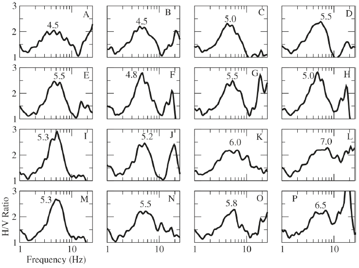
Figure 2: Mean HVSR curves of each of the recording points within the study area (Figure 1). The number within each graph indicates the maximum frequency of the HVSR, which can be interpreted as the proper frequency of vibration of the soil layer. In the upper right corner of each graph is indicated the letter denoting each measurement point
Ambient noise tomography
Noise records are usually preprocessed to retain the stationary part of the background noise (Bensen et al., 2007). In this process, an equalization of the Fourier spectrum (spectral whitening) of the noise recorded is performed so that there are contributions of the energy associated with the distinct phases. From the normalized records, we carry out cross-correlations between all pairs of receivers. In this work, we have chosen to cross-correlate windows of 60 s of overlapping duration 50 % over the 60 min of time record. In Figure 3a, we show the virtual source section 01, the result of the cross-correlation of the noise record of the receiver 01 with the remaining records of the 48 receivers. In this figure, it is observed that wave trains emerge whose amplitude is remarkable in time delays less than 1 s. The pulses have a high signal to noise ratio and emerge consistently either in the anti-causal part (times less than zero) or causal (times greater than zero). The correlation pulses between the receivers 01 and 10 show a sudden change in velocity from receiver 06. Between receivers, 10 and 19 phases and amplitude are lost in some receiver. In Figure 3b, we show the virtual source section of the receiver 25. Variations in the correlation pulse and the presence of secondary wave trains are observed in receivers 01 to 08 and 41 to 48. Moreover, at short distances (receivers 30 to 33), the correlation pulse loses its shape. Results similar to those shown in Figure 3 can be observed for the other 48 virtual source sections.
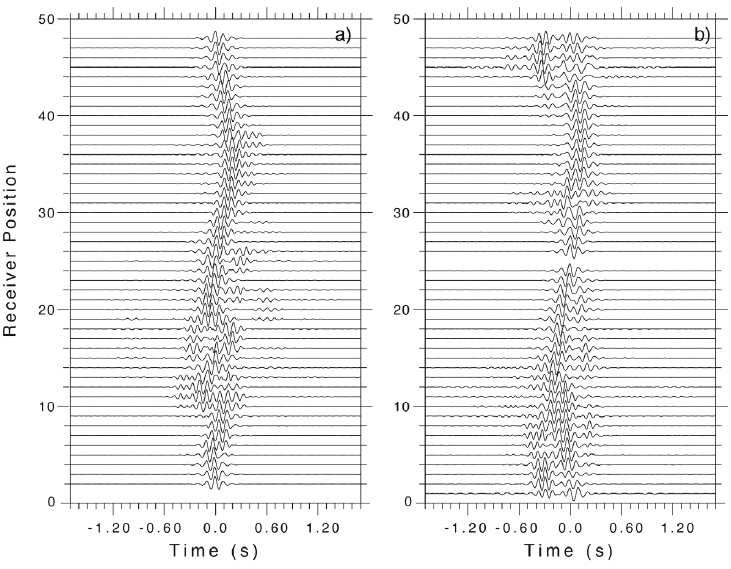
Figure 3: Virtual source sections result from the correlation of the record in receiver: a) 01 and b) 25, concerning the remaining 48. Traces are filtered between 5 and 15 Hz
The symmetry of the pulses in the cross-correlation function is related to the equipartition condition, which must be completely satisfied to obtain the EGF. This condition is fundamental in IS under the view that the wavefield in a closed system should consist of arbitrary contributions of all possible modes of propagation, with equal weight on average (Weaver & Lobkis, 1982; Schuster, 2014). If the medium contains a sufficient distribution of scatters, then it is possible to satisfy the condition of equipartition with an unique source because each scatter acts as a secondary source. In open systems, the most appropriate definition of equipartition states that the flow of energy must be equal in all directions (e.g., Snieder et al., 2007). For practical purposes, the emergence of EGF either in the causal or anti-causal part can be used to characterize the subsoil, as it is enough to add the anti-causal part to the causal part to increase the coherence of the pulse. The extraction of the correlation pulse or EGF) is because the primary source of seismic noise is due to vehicular traffic (Halliday et al., 2011) that occurs in the road circuit near the study area.
The emphasis of this study is to characterize the lateral variations of subsoil velocity. For this, we exploited the position of the delay times of the envelope maximum of the correlograms filtered in different frequencies (Cárdenas et al., 2016). The identification of travel time (maximum correlation pulse) at different frequencies can then be used to produce a tomography image that provides the distribution of the velocity of the medium separating two receivers (Shapiro et al., 2005; Sabra et al., 2005).
We used the filtered virtual source sections and extracted the maximum delay times from the envelope of the correlation pulse for 36 central frequencies generated from a mobile filter whose width is a function of the frequency for the range of 4 to 24 Hz. From those times, we built travel time tomographies to know the distribution of the group velocity. The study area was discretized by a mesh whose cells were 4 m per side, where the number of pairs of trajectories (rays) that covered the mesh, for 48 receivers (n=48), was n(n-1)/2=1128. The inversion processes were carried out by Simultaneous Interaction Reconstruction Tomographic (SIRT) method (Nolet & Wapenaar, 2009) to derive phase velocity distributions. The inversion process was further improved by incorporating the maximum slope method (Arfken et al., 1999), which minimizes the objective function. The objective function is defined as the difference between the observed data and the synthetic calculated data produced by the forward modeling, and sometimes with another term of regularization or damping (Uieda et al., 2013).
Figure 4 shows as an example, the images of the results at the frequencies of 6, 8, and 12 Hz. The color scale is different for each image to highlight the contrasts between the resolved phase velocity values. This contrast results between the mean phase velocity of 250 m/s and 500 m/s. The existence of velocity values of 250 m/s at low frequencies, such as 6 Hz, indicates that in-depth little consolidated materials prevail in the East and West of the study site. At 6 Hz, velocity values higher than 650 m/s are observed concerning the results of the images at 8 and 12 Hz. High-velocity values at low frequencies indicate the presence of more compact material in depth. A high-speed anomaly highlights at the center of the array on all three frequencies. The distribution of high velocities to the south, center, and northwest part of the array is consistent with the distribution of basaltic materials observed at the site. In general, the resolved velocity at low frequencies is higher than at intermediate and high frequencies. This behavior is characteristic of the dispersion property of surface waves, the variation of velocity as a function of frequency.
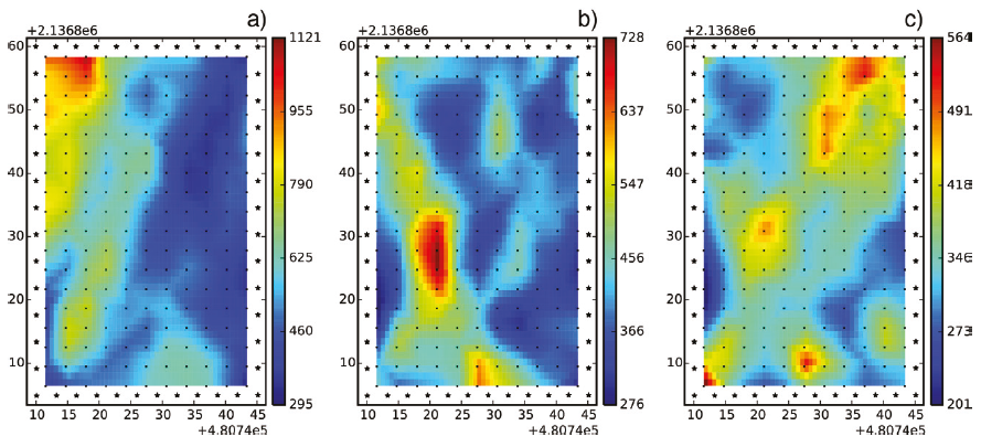
Figure 4: Seismic noise tomography at frequencies of 6, 8, and 12 Hz, a), b) and c) respectively. The phase velocity distribution (m/s) in a UTM reference system is displayed. The black stars indicate the position of the geophones. The black dots represent the Centers of the cells where the tomography method is solved. The color scale indicates the phase velocity values, and it is different for each image
The frequency-dependent velocity variation at each node of the tomography model is shown in Figure 5a. These values describe phase velocity dispersion curves of Rayleigh waves. The curves show that at frequencies close to 4 Hz (limit of the characteristic frequency of geophones), the phase velocities can be between 400 and 1400 m/s. Most curves describe velocity values between 400 and 600 m/s. for frequencies higher than 6 Hz, the decay of the curves shows values between 200 and 500 m/s. The curves shape in Figure 5a indicates they can reasonably be inverted to obtain a shear wave velocity profile. Figure 5b shows an example of the inversion of a dispersion curve (Herrmann, 2013). The procedure consisted of proposing a model of 11 layers whose thickness increases with the depth at a constant velocity (in this case, 600 m/s). After several interactions, the inversion method converges to provide a Vs velocity profile. The example in Figure 5b shows excellent convergence towards the final model.
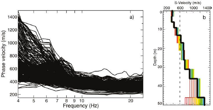
Figure 5: a) Dispersion curves obtained from travel time tomography, b) shear wave velocity profile resulting from the inversion of a dispersion curve. The discontinuous black line is the initial velocity model. The colored lines represent the different solved models until they converge to the final model (black line)
We have constructed a volume of shear wave velocity as a function of depth (Voxler 4.0 Software) from the 1D profiles resulting from the inversion of each of the dispersion curves. Figure 6 shows the 3D model of this volume, where we have highlighted two isosurfaces that describe in a general way the subsoil structure in the study area. The first of them has a value of 700 m/s and indicates the limit of poorly consolidated materials distributed heterogeneously between the surface and approximately 16 m deep. As discussed in the section on HVSR spectral ratios (Figure 2), this depth is consistent with that suggested by the 1D model of short-wave propagation (Equation 1). The depth at which the substratum is located was also determined by Sanchez (2019) from join inversion results of the HVSR and dispersion curves obtained by SPAC (Aki, 1957) and f-k (Capon, 1969) methods.

Figure 6: Shear wave velocity model produced by the interpolation of 1D Vs profiles obtained from the tomographic results. Two isosurfaces are shown; at 700 m/s (green) and 300 m/s (blue lines)
The second isosurface corresponds to the lowest velocity values (close to 300 m/s). The distribution of these values should be located close to the surface of the terrain. However, a low-velocity anomaly is observed between 10 and 20 m deep, which extends inward of the array to a distance of approximately 30 m. The anomaly coincides with an old crack located below the adjacent building. Most likely, that crack or lava tube is filled with tuffs and fractured materials. We observe that the low-velocity anomaly emerges due to inconsistent time delays of the correlation pulses. The irregularity of the correlation pulses described above suggests it is a cavity-like structure that probably causes resonance in the wave field extracted by SI (Catheline et al., 2008; Hillers et al., 2014, Argote et al., 2020).
Conclusions
The use of ambient seismic noise to characterize subsurface structure is widely used, but its applicability must consider some limitations. For example, the HVSR method works if there are significant contrasts of mechanical properties in-depth. The SI method requires an adequate azimuthal distribution of noise sources to recover the medium response adequately. These two requirements were found in the site study. HVSR spectral ratios showed a clear site response, and it was possible to extract correlation pulses due to secondary noise sources produced by the volcanic materials.
The 3D-Vs model obtained exhibits lateral and vertical variations of shear wave velocity and an irregular substratum. Although the site is geotechnically classified as firm soil, HVSR results indicate the existence of a layered structure whose surface materials produce relative amplification in the frequency range of 4.5 to 7.0 Hz. Such materials correspond to altered basalts combined with filler materials. According to HVSR peak frequencies, soft soil deposits have an average thickness of 12 m.
The cross-correlation functions extracted by SI indicate the seismic noise propagates precisely in a layered structure. In some trajectories, there are delayed or incoherent correlation pulses that define low-velocity zones. These functions correspond to Rayleigh surface waves whose dispersion characteristics allowed us to produce seismic tomography images of phase velocity in the range of 4 to 24 Hz. The 3D model built from the dispersion curves obtained from ANT shows an average velocity of 300 m/s for surface materials and 800 m/s for depths higher than 12 m. A low-velocity anomaly is also observed near the adjacent building, which correlates with an old preexistent crack or lava tube filled during the building construction.
This study shows that ambient seismic noise tomography can help define a subsoil structure model with lateral velocity variations. The model is valuable for tracking the seismic response of the site. We believe in future studies; it will also allow us to know changes in subsoil behavior to prevent damages in the building that is now is erected.
This methodology can be applied to other sites with different geological conditions. Future work includes incorporating joint inversion methods between dispersion curves and HVSR spectral ratios and improving the seismic tomography scheme for smaller arrays. It is also necessary to integrate geophysical methods like electrical tomography and gravimetry and confront the results with geotechnical studies.

