


 text new page (beta)
 English (pdf)
 Article in xml format
 Article references
 Send this article by e-mail
 Cited by SciELO
  Similars in
SciELO
Similars in
SciELO 
 Permalink
Introduction
In this article the method to calculate Prony series from DMA data will be explained with a real example. The Prony series of a piece of structural adhesive used in automotive industry will be obtained showing in detail the considerations and background of each decision taken during the analysis with the purpose of being a good reference for the reader. The motivation for writing this article is the lack of literature available on this subject.
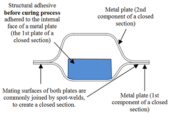
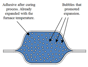
Background on this article analysis is as follows: Automotive body is manufactured from steel or aluminum plates (Davies, 2003). Structural adhesives are used to fill the cavities between these plates and therefore increasing the strength of the structure. Normally they are installed before paint process as it is shown in Figure 1, where they will be cured with the furnace temperature. The installation process consists on place them on the surface of a metal plate in order they adhere by themselves to it. This process is most of the times done manually by an operator. Some of these adhesives when heated liberate gases that will create small bubbles on them, and they will increase their volumes, this is the expansion mechanism that promotes the filling of the closed section in the body structure as shown in Figure 2.
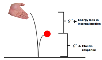
Energy during the impact will be dissipated by the structural adhesives. The properties that describe the energy dissipation capacity of materials are known as dynamic properties. The complex modulus G* is a complex quantity that can be divided in a real part and an imaginary part, called storage modulus G', and the loss modulus G'', respectively. Their relationship is indicated in equation 1.
The storage modulus G' describes the capacity of a material of storing and returning energy to the surroundings, and the loss modulus G'' describes the capacity of a material of dissipating energy on its internal structure. A graphical explanation of these concepts are often explained with the Figure 3.
Dynamical mechanical analysis
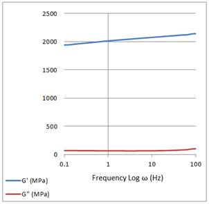
The dynamical properties are obtained by an experimental method called dynamical mechanical analysis, DMA from now on. DMA is performed in a laboratory using a Dynamic Mechanical Analyzer, a device commonly used in the study of polymers rheology. Dynamical properties are studied by applying a cyclic stress into a material sample (Sepe, 1998), it can be applied in different modes: tension, bending, cantilever, dual cantilever, torsional, etc. Often the results are shown as frequency response diagrams, also named frequency sweep, where in the vertical axis are shown the values of Storage Modulus G' and loss Modulus G'', and in the horizontal axis are shown the frequencies where the analysis was performed. Most of the times horizontal axis is presented in a logarithmical scale since it is important to show high and low frequency values. An example of a frequency scan can be observed in Figure 4.
The Dynamical Mechanical Analyzer is a device that has movable and fixed clamps. The fixed clamps remain static while the movable clamp will be displaced up and down by a driveshaft deforming the material in an oscillation pattern as illustrated in Figure 5. The amplitude and frequency of the oscillation is programed based on the characteristics of each material. The mathematical background for the calculation of G' and G'' can be found in (Ferry, 1980).
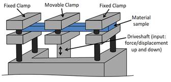
In this work a sample of cured structural adhesive (epoxy) with low expansion capability (around 15 % of volume increase) was evaluated. Frequency sweep from 0.1 to 100 Hz was carried out with a Q800 TA Instrument DMA device using a dual cantilever clamp configuration as is shown in Figure 5. An oscillation amplitude of 5 mm was applied at a constant temperature of 30 °C to obtain the experimental viscoelastic properties. Structural adhesive sample dimensions for dual cantilever DMA test were 35.0x13.1x3.7 mm. These samples were prepared cutting the sample of epoxy adhesive with the required dimensions and cured in a convection furnace at 120 °C for 2 hours. Structural adhesives can go from a 15 % to a 300 % expansion ratio depending on the application and performance required. DMA is performed in order to obtain the values of G', G'' and tanδ that is defined as:
In a DMA experiment where a cyclic force is applied on a material sample, it can be noticed a phase lag between the applied load curve and the strain curve, as shown in Figure 6. This phase lag is an angle named δ. tan δ is a quantity often used in polymers rheology, also known as damping factor and it is related to the energy that the material is dissipating on its structure.
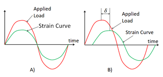
Figure 6: Explanation of tan δ concept: a) shows the plots of an ideal 100 % elastic material, where both curves are in phase, b) shows the plots of a viscoelastic material where there is a phase lag between both curves
The method used to get the dynamical properties of the structural adhesive was the following: the imposed deformation mode was dual cantilever, and the size of the sample was 35.0x13.1x3.7mm. The analysis was performed in a range of frequencies that goes from 0.1 to 100 Hz, with 10 measurements on each frequency decade. A decade must be understood as an order of magnitude, for example; from 0.1 to 1 we have 1 decade and from 1 to 10 we have another one. This frequencies range was selected based on vibrations commonly detected in automotive bodies due to the input of pavement irregularities through vehicle’s suspension. That input typically goes from 1 to 2 Hz, as mentioned in (Spinola, 2012), nevertheless it was decided to measure in a wider range in order to have the necessary data to make the curve approximation of G' or G'' as functions of the frequency 𝜔 as it will be exposed later in this work.
It is desirable to have a wide range of measurements along 3 or more frequency decades for any material under study to have a good material characterization. Also it is recommended that the common usage input frequency of the product that is under study is included in this range (in this case the structural adhesive used in automotive body). The advantage of perform testing in the frequencies domain is that it requires less time than carry out them on time domain, since the frequency is an inverse quantity with regards of time. This characterization in the frequencies domain will allow a good curve fitting that will let us know the numerical values that will be finally substituted in the Prony series that are functions in the time domain.
The deformation applied to the sample depends on the nature of the material. One method is to impose a small deformation (less than 1 % of the sample size) and keep increasing it until a constant value of the moduli is obtained.
The measured values obtained by performing DMA to this sample are shown in the Table 1.
Table 1: Data obtained from DMA
| Time | Temperature | Frequency | Storage Modulus |
Loss Modulus |
Tan Delta |
Angular Strain |
| min | °C | Hz | MPa | MPa | % | |
| 7.49 | 30.26 | 0.1 | 1941 | 70.08 | 0.03611 | 0.08203 |
| 16.95 | 30.19 | 0.13 | 1944 | 70.48 | 0.03626 | 0.082 |
| 24.06 | 30 | 0.16 | 1953 | 69.81 | 0.03574 | 0.082 |
| 25.81 | 30 | 0.2 | 1961 | 68.64 | 0.035 | 0.08202 |
| 27.8 | 30 | 0.25 | 1968 | 68.17 | 0.03463 | 0.08202 |
| 32.92 | 30 | 0.32 | 1976 | 67.41 | 0.03411 | 0.08201 |
| 34.66 | 30.01 | 0.4 | 1983 | 67.03 | 0.03379 | 0.08202 |
| 35.74 | 30 | 0.5 | 1990 | 66.37 | 0.03335 | 0.08202 |
| 45.19 | 30 | 0.63 | 1998 | 65.99 | 0.03302 | 0.08201 |
| 56.9 | 30 | 0.79 | 2007 | 65.61 | 0.0327 | 0.08201 |
| 59.52 | 30 | 1 | 2014 | 65.14 | 0.03234 | 0.08203 |
| 60.5 | 30 | 1.3 | 2021 | 64.65 | 0.03199 | 0.08202 |
| 61.7 | 30 | 1.6 | 2027 | 64.54 | 0.03184 | 0.08202 |
| 62.08 | 30 | 2 | 2033 | 64.26 | 0.0316 | 0.08203 |
| 62.32 | 30 | 2.5 | 2039 | 64.04 | 0.0314 | 0.08203 |
| 63.33 | 30 | 3.2 | 2046 | 63.56 | 0.03106 | 0.08202 |
| 63.7 | 30.01 | 5 | 2058 | 64.16 | 0.03118 | 0.08203 |
| 64.68 | 30 | 6.3 | 2064 | 64.53 | 0.03127 | 0.08203 |
| 65.88 | 30 | 7.9 | 2069 | 64.9 | 0.03136 | 0.08203 |
| 66.26 | 30 | 10 | 2076 | 65.59 | 0.0316 | 0.08203 |
| 66.78 | 30 | 12.6 | 2082 | 66.4 | 0.0319 | 0.08203 |
| 67.4 | 30 | 15.8 | 2087 | 67.69 | 0.03243 | 0.08203 |
| 67.65 | 30 | 19 | 2093 | 68.91 | 0.03293 | 0.08203 |
| 67.8 | 30 | 25 | 2100 | 71.17 | 0.03389 | 0.08203 |
| 68.32 | 30 | 31.6 | 2106 | 73.72 | 0.035 | 0.08203 |
| 68.94 | 30 | 39.8 | 2112 | 76.72 | 0.03632 | 0.08203 |
| 69.19 | 30 | 50 | 2119 | 81.4 | 0.03842 | 0.08203 |
| 69.34 | 30 | 63 | 2121 | 85.96 | 0.04053 | 0.08203 |
| 69.59 | 30 | 79.5 | 2137 | 97.34 | 0.04556 | 0.08203 |
| 69.76 | 30 | 100 | 2141 | 102.3 | 0.04779 | 0.08203 |
Models of viscoelastic behavior
Most of all materials have a viscoelastic behavior and in the case of adhesives it is remarkable due to their polymeric nature. Elastic behavior is modeled by Hooke law that can be represented by the following equations:
In the case of tensile stress, and:
In the case of shearing stress; where:
σ = |
tensile stress |
E = |
Young’s modulus |
ε = |
tensile strain |
τ = |
shear stress |
G = |
shear modulus |
γ = |
strain by shear |
Viscous behavior is modeled by the Newton’s law:
In the case of viscoelasticity of polymers, a more complex model is needed because it depends on several facts: the size of the molecules, if they are crosslinked or not (Ferry, 1980), and also stress relaxation due to polymeric chains re-ordering with time. By these reasons, the equation that models viscoelasticity uses a modulus that is a function of time, as follows:
Where G(t) is the stress relaxation modulus of the material.
Ferry (1980) shows the same constitutive equation with the following notation:
Where:
σij = |
stress tensor |
|
strain rate tensor |
t' = |
all the past times were the integration must be carried out over all of them, this must be considered due to the memory of the material during deformation. |
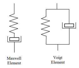
Two basic mechanical models that predict viscoelastic properties of materials are Voigt and Maxwell elements, that are represented by springs and dashpots connected between them, as illustrated in Figure 7. The materials behavior can be described as combinations of Maxwell and Voigt elements connected between them. One simple model is the generalized Maxwell model that is just a set of Maxwell elements connected in parallel.
In generalized Maxwell model, the contribution in relaxation modulus of each Maxwell element is given by the equation 8:
Where Gi is the spring constant and τi is the relaxation time of the element, defined in equation 9.
Where ηi is the dashpot constant. The relaxation modulus of the complete model is the sum of the relaxation moduli of all Maxwell elements connected in parallel, as follows:
When t→∞ in the case of materials that have a solid-like behavior, G(t) approaches a finite value Ge. For liquid-like materials, G(t) approaches zero (Ferry, 1980), this is why in the case of structural adhesives, that become solid-like materials after the curing process, the equation 4 can be rewritten as:
The equation 11 is also known as the Prony Series (Tschoegl, 1989) of the material, and is useful to describe viscoelastic properties in CAE Software (ABAQUS, 1998).
Using DMA data to get Prony series of structural adhesives
As mentioned previously, it is possible to obtain the values of storage modulus G' and loss modulus G'' in function of the frequency by performing DMA to a sample of material. Also, as exposed by Ferry (1980) & Tschoegl (1989), these quantities are represented as functions of frequency in the following equations:
This means that is possible to make a curve approximation in order to know the values of the Gi and τi terms, depending on the number of terms desired for the sum. One theoretical method is exposed by Baumgaertel & Winter in (1989). For practical uses, this can be done using software to approximate the curve to these custom equations. The first step is to decide the number of terms. For this work, we will approximate a curve to the first two terms of the sum shown in equation 12.
In equation 14 there are five unknown values: Ge, G1, G2, τ1 and τ2, these values will be approximated by fitting the curve with the form of equation 14 to the data obtained by DMA on the “Storage Modulus” column in Table 1. Software such as Matlab® can be used for a fast procedure capable to meet the Automotive Industry demands on quick analysis. The command used in Matlab® to make the curve approximation is “cftool” (curve fitting tool). This command will display an interactive fitting tool where the column vectors previously created with the information of the columns “Storage Modulus” and “Frequency” in the Table 1 can be loaded as vertical and horizontal axis respectively. In the case of solid-like materials is convenient to use the storage modulus instead of the loss modulus, for example, in this material it was possible to make the approximation of the curve with 30 points over 3 decades, but in the case of loss modulus the experiment should be made in a wider range of frequencies to get a better approximation of loss modulus curve. The loss modulus values are small in comparison to storage modulus values (by a factor of 30 times approximately). This also can be noticed in tanδ values that approach zero. By this reason it is very difficult to get a good approximation with loss modulus curve, since dominant behavior is described by storage modulus. Only storage modulus curve approximation will be discussed in this work.
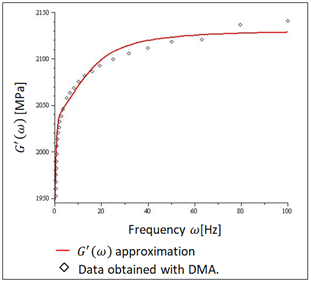
The obtained values from storage modulus G'(ω) curve approximation are the following: Ge=1947.00, G1=85.79, G2=97.63, τ1=0.0659, τ2=1.6950, replacing these values in equation 14 it is obtained a function of the frequency ω only, as is shown in equation 15:
By plotting the equation 15 as a function of the frequency 𝜔 is obtained the chart in Figure 8:
The values obtained in the curve approximation can also be replaced in the equation 11, in this case for the two first terms of the series, obtaining:
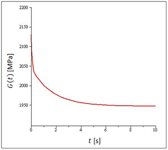
The terms of equation 16 are the Prony series of the structural adhesive, also known as the relaxation modulus of the material in function of time. In Figure 9 is showed a plot of equation 16 as a function of time t, it is possible to observe the behavior of the relaxation modulus, where can be noticed that it’s value when a load have been applied for a long time tends to the value of Ge=1947.00 MPa, as mentioned previously.
It can be confirmed the accuracy of the model since the approximated values of G'(ω) calculated with equation 15 have less than 1 % of error with regards of the data obtained by experimental measurement through DMA experiment. Table 2 shows the error calculation for each DMA data point vs. the calculated value with the approximated function.
Table 2: Error calculation of values measured with DMA vs. values calculated with the fitted function G'(ω) (equation 15)
| Frecuency | Calculated storage modulus with equation 15 |
Measured storage modulus |
|
| Hz | MPa | MPa | % |
| 0.1 | 1949.7303 | 1941 | 0.4498 |
| 0.13 | 1951.5271 | 1944 | 0.3872 |
| 0.16 | 1953.6981 | 1953 | 0.0357 |
| 0.2 | 1957.0780 | 1961 | 0.2000 |
| 0.25 | 1961.882 | 1968 | 0.3107 |
| 0.32 | 1969.2311 | 1976 | 0.3426 |
| 0.4 | 1977.8047 | 1983 | 0.2620 |
| 0.5 | 1987.9030 | 1990 | 0.1054 |
| 0.63 | 1999.1612 | 1998 | 0.0581 |
| 0.79 | 2009.9052 | 2007 | 0.1448 |
| 1 | 2019.7899 | 2014 | 0.2875 |
| 1.3 | 2028.5758 | 2021 | 0.3749 |
| 1.6 | 2033.8793 | 2027 | 0.3394 |
| 2 | 2038.2660 | 2033 | 0.2590 |
| 2.5 | 2041.7259 | 2039 | 0.1337 |
| 3.2 | 2045.0396 | 2046 | 0.0469 |
| 5 | 2051.6141 | 2058 | 0.3103 |
| 6.3 | 2056.2783 | 2064 | 0.3741 |
| 7.9 | 2062.2139 | 2069 | 0.3280 |
| 10 | 2070.0282 | 2076 | 0.2877 |
| 12.6 | 2079.1046 | 2082 | 0.1391 |
| 15.8 | 2088.7098 | 2087 | 0.0819 |
| 19 | 2096.4331 | 2093 | 0.1640 |
| 25 | 2106.6909 | 2100 | 0.3186 |
| 31.6 | 2113.6681 | 2106 | 0.3641 |
| 39.8 | 2118.8206 | 2112 | 0.3229 |
| 50 | 2122.4477 | 2119 | 0.1627 |
| 63 | 2124.9605 | 2121 | 0.1867 |
| 79.5 | 2126.6367 | 2137 | 0.4849 |
| 100 | 2127.7134 | 2141 | 0.6206 |
These results allow us to confirm that model showed in equation 15 is a good prediction for G'(ω) since the error values are below 1 %, and this assure that G(t) values will have good correlation with real behavior.
CAE modeling using Prony series
As mentioned previously, the Prony Series of equation 16, are also known as the discrete relaxation modulus in function of time. When equation 16 is substituted in equation 7, the constitutive equation is completely defined, the resulting equation is:
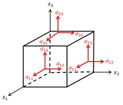
CAE makes possible to incorporate the geometry of the product under analysis by dividing a complex geometry in small elements through the creation of a mesh. Equation 17 will be discretized and solved for each one of the elements of this mesh, since σij is the stress tensor of an infinitesimal element as ilustrated in Figure 10.
The definition of Prony Series may be different on each commercial CAE software package. In the case of Abaqus® when the model is viscoelastic and defined in the time domain, the software displays a table similar to Table 3, where the requested parameters are: gi, ki, and τi. The gi terms are the normalized Prony coefficients for shear (deviatoric) behavior, the ki terms are the normalized Prony coefficients for volumetric behavior, and the τi values are the relaxation times of Prony series. Abaqus® assumes that the frequency dependence of gi and ki is independent. In this work the volume changes in the material will not be considered, therefore the column for ki values will be left blank. The changes in shape are described by the deviatoric behavior, described by gi terms, they are defined as follows (Chen, 2000):
Table 3: Dimensionless Prony series coefficients input in Abaqus®
| g1 | k1 | τi |
| 0.0403 | - | 0.0659 |
| 0.0458 | - | 1.695 |
Where the Gi values are the coefficients of the Prony series, and G0 is the relaxation modulus G(t) evaluated in t=0.
Calculating the values of G0, g1 and g2:
g1 and g2 are also known as the dimensionless Prony series coefficients.
Table 3 shows the input of values in Abaqus®. This table can have as many rows as known terms of the Prony series are available. By filling this table, the viscoelastic characteristics of the material under study are completely defined.
The method to calculate the relaxation modulus in function of time presented in this work has many application possibilities. Examples of other applications in automotive industry that used Prony series to describe viscoelastic behavior are : Prediction of damping of railway sandwich type dampers (Merideno et al., 2014), Modeling of viscoelastic parameters for automotive seating applications (Deng et al., 2003), Stress concentration analysis near holes in viscoelastic bodies (Levin et al., 2013), Analysis of adhesion of thermoplastics to steel (Golaz et al., 2011), Finite element analysis of seat cushion and soft-tissue materials focused on passenger-vehicle occupants comfort (Grujicic et al., 2009), Modeling of composites viscoelastic behavior (Machado et al., 2016; Ishikawa et al., 2018).
Conclusions
Viscoelastic properties of materials applied on CAE studies can provide more accurate results since it is a better approximation to real behavior of the material. The relaxation modulus of the analyzed structural adhesive showed a significant dependence with time since modulus values change from the maximum value in G0=2130.42 MPa to the value of Ge=1949.00 MPa due to stress relaxation. This shows that for vehicle CAE impact evaluation that occurs at a high speed the modulus will have also a high value since the stress relaxation will not occur at this speed. In the case of durability CAE evaluation, where the load is applied in long periods of time or in a time dependant load variation the stress relaxation will occur, therefore the modulus value will achieve the Ge value. Viscoelastic properties of structural adhesives can be incorporated to CAE by estimating Relaxation modulus in function of time through Prony series by fitting a model to DMA experimental data in function of frequency.
Model fitting for G'(ω) with respect to experimental DMA data showed an error smaller than 1 % using only two terms of the Prony series.
Through this methodology, parameters required to model viscoelasticity behavior in function of time in CAE software like Abaqus® can be obtained from the information of a single DMA experiment performed to a small material sample.

