


 text new page (beta)
 English (pdf)
 Article in xml format
 Article references
 Send this article by e-mail
 Cited by SciELO
  Similars in
SciELO
Similars in
SciELO 
 Permalink
Introduction
The necessity of a better control management at intersections (through traffic lights) and a suitable route guidance approach increases along with the vehicles increment on streets. The present study explores adaptive solutions to improve the traffic quality: an auto-regulated control at intersections, which sets the traffic lights times and has the purpose to relieve the streets with more vehicles, and a route choosing algorithm, with the intention to guide the vehicles through the streets with the least quantity of vehicles and reach the destination faster.
There is work related with adaptive traffic lights. In Gershenson & Rosenblueth (2012b) the traffic lights adjust its times according the vehicles demand, the streets are fragmented in cells and elementary cellular automata rules are applied, an algorithm with rules is implemented that basically counts the number of vehicles within a distance before the intersection, the street which count exceeds a threshold gets the green, also rules are implemented to prevent that streets with a bottleneck (occurring after the traffic light location) get the green, the self-organizing method shows better average speed and average flow, at different densities, than fixed traffic lights. In Gershenson (2004), with multi-agent simulations, three self-organizing methods are tested against traditional, the variables measured were: number of stopped cars, the average speed and average waiting times. The self-organizing methods implemented were: Sotl-request control, which counts vehicles to select the street with priority, Sotl-phase control, same as Sotl-request but with a minimum time imposed to terminate the green time, and Sotl-platoon control, in which platoons with no more than µ vehicles can pass before changing to red. These methods are self-organizing since the rules independently regulate each intersection, and despite that, global coordination is achieved. Self-organizing methods outperformed traditional control methods due its adaptive nature (instead of optimizing), also is concluded that the formation of platoons minimizes conflicts among vehicles. In De Gier et al. (2011) is shown the better performance of adaptive traffic lights against non-adaptive, the travel time mean and fluctuation is lesser in the adaptive case if the system is informed of the traffic situation in the upstream and downstream links, in contrast to have only the information of the upstream links. In Fouladvand et al. (2004) is proposed a traffic responsive signalization algorithm, following the concept of cut-off queue length and cut-off density, where is wanted to reduce the total delay of the intersecting streets, leading to the optimum signalization. The work in Gershenson & Rosenblueth (2012a) shows that using a self-organizing method the traffic lights control on cities can be improved for the drivers benefit. In Helbing et al. (2005) it is presented a fluid dynamic model to simulate traffic on roads with different lengths and capacities, the model is designed to easily simulate congested and free traffic, also throughputs and travel times are improved considering self-organization principles to set the interaction between vehicles and traffic lights. In Lämmer & Helbing (2008) is introduced an approach to coordinate incompatible traffic flow at intersections based on observed pedestrian flow activity (people walking), with optimization and stabilization rules, the self-organized control presents a low performance if the road neatwork is being used a lot, being necessary a proper combination to get a high performance (reduction of travel time and its variation). In Carrillo et al. (2018) is presented an algorithm that regulates the traffic at an intersection, without the need of traffic lights, keeping a balance in the number of vehicles passing from each direction, adequate for streets where no side has priority.
There is also work related between self-organization and traffic. The self-organization effects in the high and low density traffic flow phases are studied in Biham et al. (1992), where with a simple model the traffic flow is described. A self-organized traffic information system is proposed in Wischoff et al. (2003), where vehicles perform traffic analysis and the information is shared with other vehicles. In Viriyasitavat & Tonguz (2012) is proposed a management scheme that delegates the function of regulating the traffic to a leader vehicle, which serves as a virtual traffic light. With a set of rules, the priority of emergency vehicles is established, the simulations show that the emergency vehicles travel time is reduced, and the other vehicles travel time is not significant affected. In Tonguz et al. (2011) is presented a biologically inspired approach to solve transportation problems using the self-organizing paradigm.
The cause of driving accidents is usually due human mistakes, with autonomous vehicles (AVs) is intended to replace the human intervention, but some problems arises, as the design of a control to manage the AVs. The current study proposes a solution to achieve a safety driving interaction among AVs, and these with a human controlled vehicle. These findings contribute with knowledge to the intelligent traffic field. In Nagel et al. (2006), an algorithm that allows path planning and obstacle avoidance at 132 miles of unknown and rough territory is introduced. In Liao (2012), a modification of the A* algorithm in order to avoid collisions among unmanned aerial vehicles (UAVs) is presented. Wei & Dolan (2009) focus on autonomous driving, a prediction engine (for anticipating the intentions of the surrounding vehicles), a cost function based scenario evaluation (that evaluates the predicted scenarios and generates strategies), a cost function based algorithm (used in driving ability, distance keeping, lane selecting and merge planning) and a freeway driving performance analysis (that combines qualitative and quantitative performance evaluations) were implemented. In Resende & Nashashibi (2010), two methods for real time trajectory planning, applied to automated driving and implemented for the HAVEit European project, are presented. First method considers the partial motion planning approach, and the second employs a fifth-degree polynomial to generate the trajectory (the coordinates to perform a lane change at constant speed). In Qian et al. (2014), is proposed that legacy vehicles (manually driven) respect car following rules to achieve the driving interactions between AVs and legacy vehicles.
Intersection control
The simulations conducted in this article were developed in the Unity Engine (Technologies, n.d.). The travel time (Yu-qin et al., 2013) to cross a road segment is slightly modified and presented in Equation 1.
The author exchange flow per density in Equation 1, from which
where l is the road segment length. In this study a road segment (or street segment) starts and ends with an intersection, and each segment measures 1000 m. A vehicle’s travel time (T) is set using Equation 1 with D as the number of vehicles circulating ahead, e.g. if there is a platoon of 3 vehicles approaching the segment, the travel time of the 1st vehicle arriving on the segment is calculated with D=1, the 2nd vehicle with D=2 and so on, therefore T modifies the vehicles speed through Equation 2. A vehicle’s speed is recalculated (this apply for each vehicle on the segment) when a vehicle leaves or arrives at the segment, because the travel time depends of D and this variable is refreshed as the number of vehicles in front of the current vehicle.
The control logic is designed accounting for the number of vehicles on the segments, i.e. a segment with more vehicles, should has the priority. The meaning of the variables and constants employed are presented in Table 1. The letters a and b are used (interchangeable) for referring any two intersecting segments which traffic flow is related with traffic lights, in this case the south-north flow direction segment with east-west, and south-north with west-east. The capacity density on any segment is C a =C b =C=1vehicle/5m=200 vehicles/1000 m, as previous defined.
Consider now P
ab
(see Equation 3), which is the difference of the ratios
If
Otherwise, if
The case when
Simulations results
The first scenario to conduct simulations has two intersections, as presented in Figure 1, with three flow directions: down-up (south-north) in blue arrow, right-left (east-west) in red arrow and, left-right (west-east) in orange arrow.

Two simulations were performed using the scenario presented in Figure 1: adaptive control vs. conventional control. The conditions for both simulations were the same: the vehicles from south-north were generated each 1 s, from east-west each 2 s and west-east each 3s. As mentioned before, the street segments length is 1000 m, and the traffic capacity (per segment) is C = 200 veh / 1000 m. The control points, to stop the vehicles if
Table 2 Number of vehicles passing through the intersection(s)
| South-north | East-west | West-east | Total | |
|---|---|---|---|---|
| Conventional | 412 veh* | 258 veh | 172 veh | 842 veh |
| Adaptive | 462 veh | 255 veh | 172 veh | 889 veh |
*veh=vehicles
A scenario with one intersection and four traveling directions (Figure 2) was implemented for the next simulations. Defining Ts as the time between vehicles arrivals, the vehicles from the south-north direction (in blue arrow) were generated each Ts=0.5 s, from north-south (yellow arrow) Ts=1 s, from east-west (red arrow) Ts=3.5 s, and from west-east (orange arrow) Ts=4 s, the simulation time was 300 s, other configurations remain the same.

Two simulations were performed, adaptive vs. conventional control. The number of vehicles passing the intersection is greater for the adaptive control (Table 3), with an improvement of 111 vehicles. The green time assigned to allow the flow from south-north and north-south directions (those with more vehicles circulating) in the conventional control is not enough, as the adaptive control simulation results suggest, with more vehicles passing the intersection from the directions mentioned before.
Route guidance
A solution to reduce the vehicles travel time is to distribute (with an adaptive paradigm) the vehicles along the streets, from the arriving to the destination place. The routing algorithm (Annex A) was designed to establish a route with low density streets. The algorithm seeks for the streets that conform a route solution and with density<threshold. The threshold initial value is the lowest defined, if no solution is found, the threshold value is incremented, this process continues until a solution is found. For simplicity, the street network selected for simulating purposes has a grid form, with four blocks (Figure 3). If a vehicle’s departure location is in the below-right corner and the destination location in the upper-left, with the horizontal streets with a flow direction from east-west and the vertical streets with flow from south-north, the route solution should involve to travel two segments to the left and two to the top, then there are six possible solutions as presented in Table 4, with u=up and l=left. The number of vehicles traveling on a street segment (Figure 3 shows the segment labels) is used to assign a weight to it, understanding that the more weight a segment has, it is harder to travel on it.

Simulation results
In this simulation the time cycle of the traffic lights (to regulate the traffic at intersections) is fixed (conventional control). A vehicle is created each 0.5 s in the origin, the intersection between l1,1 and u1,1. The first 120 vehicles follow pre-defined paths: these go through the u1,1 segment, then are distributed equally between u1,2 and l2,1, continuing with l3,1 and u2,2, respectively. The path of the vehicle 121 is defined with the routing algorithm. Figure 4 shows a two-dimensional plane, with units in meters. It can be seen in red the trajectory of the vehicle 120, which follows the defined path u1,1, u1,2, l3,1, and l3,2. The trajectory in blue is the followed by the vehicle 121, which path is l1,1, l1,2, u3,1, and u3,2, and was selected with the routing algorithm. Table 5 shows the vehicles entrance time (to u1,1 and l1,1 for vehicles 120 and 121, respectively) and the vehicles leaving time (by l3,2 and u3,2 for vehicles 120 and 121, respectively). In this simulation the travel time improvement of the vehicle guided (121) vs. not guided (120) is 14.86 s, this value is the difference between the travel times in Table 5. In this table, the entering and leaving time values represent the time in seconds (time=0 when the simulations starts) when a vehicle enters and leaves the street network, respectively. The travel time is the difference of the exit and entrance time. This result suggests that the routing algorithm effectively avoids streets with high density.

Autonomous vehicles interactions
In this section were performed simulations where the AVs interacts with each other without collisions, with this purpose an algorithm was proposed, in addition additional rules were implemented to allow the participation of a vehicle manually controlled. The braking algorithm (annex B) was employed to control the vehicles acceleration (deceleration) in the simulations from this section. The algorithm basically calculates the intersecting coordinates (if any) among the AVs trajectories, then selects the order for the AVs to accelerate or decelerate, avoiding conflicts. In the case where a manually controlled vehicle participates, the algorithm estimates the possible trajectory of this vehicle (based on the past coordinates), subsequently determines if the trajectories of the AVs and the manually controlled vehicle intersects, in that case regulates the acceleration (deceleration) of the AVs to allow the free-driving of the manually controlled vehicle.
Simulation 1
In this simulation, the AVs maximum speed (v m ) is 10 m/s, maximum acceleration a m = 2 m/s2 and maximum deceleration d m = -2 m/s2. Three AVs participates, which trajectories intersect in the same coordinate. As initial conditions, the AVs are stopped (Figure 5), the destination coordinates (or targets) are the points with the same color of the AVs, the black vehicle is the manually controlled vehicle (abbreviated CV and has no participation in this simulation). The AVs are numbered as next: red vehicle (or car) the 1st, orange vehicle the 2nd and, green vehicle the 3rd. When the simulation starts, the vehicles accelerate and follow its respective trajectory, later the 1st and 3rd vehicles decelerate because the 2nd vehicle has priority (assigned with the braking algorithm), see Figure 6.


After the 2nd vehicle has passed the conflict coordinate (where the vehicles trajectories intersect), the priority is assigned to the 1st vehicle, as can be seen in Figure 7. Finally, all the vehicles reach their target.

The variables of each vehicle involved in the simulation are presented in plots to explain how the braking algorithm operates. A vehicle without priority accelerates (if is the next in the priority queue) when the vehicle with priority has passed the conflict zone, i.e. the coordinate where their trajectories intersect. The plots that explain the simulation are presented next. In this simulation, node1 is the intersection coordinate between the 1st and 2nd vehicles trajectories, node2 is the intersection of the 1st and 3rd vehicles, and node3 is the intersection between the 2nd and 3rd vehicles. In addition, the target of the 1st vehicle is called target1, and so on for the other vehicles.
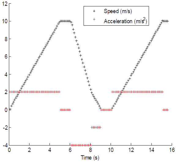
Figure 8 shows the variables evolution of the 1st vehicle: the 2nd vehicle is arriving first at node1 than the 1st vehicle, this induces the braking of the 1st vehicle when the braking distance plus an aggregated distance (to stop with anticipation) becomes larger than the distance of the 1st vehicle with node1, this happens in time approximately at 6.67 s. The braking distance =

Figure 9 shows the variables evolution of the 2nd vehicle: the trajectory of the 2nd vehicle is not interrupted by any other vehicle, it can be observed that the acceleration is zero when its speed is at maximum (10 m/s), and only decelerates when the braking distance is larger than the distance with its target, at 10.06 s.

Figure 10 shows the variables evolution of the 3rd vehicle: this decelerates at 6.67 s because the 2nd vehicle has priority and the braking distance plus the aggregated distance is larger than the distance of the 3rd vehicle with node3, eventually at 7.72 s the 2nd vehicle passes node3. As the 1st vehicle has priority over the 3rd, the 1st vehicle passes node2 at 9.80 s and enables the 3rd vehicle to accelerate. Finally, this decelerates to reach its destination at 15.99 s, because the braking distance is larger than the distance between the 3rd vehicle and target3.

Simulation 2
In this simulation, the manually controlled vehicle participates. The Lagrange interpolation technique was considered for estimating the future coordinates of the CV, the formula is presented in Equation 6.
where
The time is the independent variable used for estimating the future CV coordinates (
The estimated intersecting coordinate
The CV is manipulated with the keyboard using the direction keys, if the “up arrow” key is pressed, the vehicle accelerates continuously 2 m/s2 until the button is released, with the “down arrow” key decelerates -2 m/s2, the “right arrow” key rotates the vehicle by 0.8 degrees to the right and in the opposite direction if the “left arrow” key is pressed.
The initial vehicles position is presented in Figure 11. The trajectory followed by the CV (a straight line in the south-north direction) first causes the deceleration of the 3rd vehicle, later induces the braking of the 2nd vehicle and this causes the braking of all the AVs (Figure 12). A node is referred as the collision coordinate between the controlled vehicle and an autonomous vehicle: node1 is the collision coordinate (CC) between the controlled vehicle and the 1st autonomous vehicle, node2 is the CC between the CV and the 2nd AV, and so on. In this simulation the braking distance =
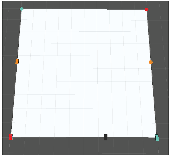

Figure 13 shows the variables evolution of the 3rd vehicle: at 4.8 s the 3rd vehicle decelerates because two rules: 1) the braking distance is larger than the distance from the 3rd vehicle to node3 and, 2) the required time to reach node3 by the CV is lesser than by the 3rd vehicle. The 3rd vehicle decelerates until the CV passes node3 (plus 5 m) at 7.59 s, also decelerates at 9.61 s because the CV causes a bottleneck. The 2nd vehicle stops (because the CV obstructs its trajectory), this induces the braking of the 1st and 3rd vehicles. The 3rd vehicle accelerates when the 1st vehicle is not obstructing its trajectory anymore and finally decelerates because the proximity of its destination.

Figure 14 shows the variables evolution of the 2nd vehicle: at 5.82 s the 2nd vehicle decelerates because the time to arrive to node2 by the CV (3.19 s) is lesser than the required by the 2nd vehicle (3.79 s). Then at the 17.92 s, the CV passes node2 over 5 m, allowing the 2nd vehicle to accelerate, finally at the 22.51 s the 2nd vehicle decelerates because it is arriving to its destination.

Figure 15 shows the variables evolution of the 1st vehicle: this decelerates at the 7.09 s due the bottleneck caused by the CV, at the 18.98 s the bottleneck ends and the 1st vehicle is able to accelerate, then at the 21.76 s decelerates because the CV intercepts its path. The deceleration rules are: the braking distance is larger than the distance from the 1st vehicle to node1, the distance from the CV to node1 is lesser than 5 m, and the time of the CV to reach node1 is lesser than the required by the 1st vehicle. An advantage rule is always considered; the CV is 5 m closer (than actually is) and the AVs are 5 m away (than actually are) of the collision coordinate (or node), subsequently the time required by the CV to reach a node is zero when it is at least by 5 m 8or closer) from the node. The 1st vehicle accelerates when the CV has passed node1 by 5 m and later decelerates due the destination proximity.

Simulation 3
In this simulation the future position (1 s ahead of the current time) of the CV, using three previous position samples, is estimated. If it is detected that the trajectory (including the estimated future position) of the CV intersects the trajectory of an AV and a collision will occur, measures are taken to decelerate (opportunely) the AV. Figure 16 shows: the estimated intersecting coordinate (IC), which is the collision coordinate between the CV and an AV considering the CV future position, and the current intersecting coordinate, which is the collision coordinate of the vehicles current linear trajectories.

Additional rules are introduced: if the AV is closeness in distance to the estimated intersecting coordinate, then it is concluded that the collision will occur in the IC, if not, will occur in the current intersecting coordinate. For the case of the collision occurring in the IC: if the CV can arrive (determined with the calculation function, in Annex B) at the collision coordinate in 5 s (or less) and the AV distance to arrive at the CC is lesser than the distance to brake =

Conclusions
Adaptive solutions for two problems were tested: 1) setting the traffic lights times and 2) choosing optimal routes, both suitable to manage autonomous traffic, however combining these (out of the scope in this study) a major benefit is expected.
With the procedure presented in the intersection control section, the traffic light times of intersecting streets are effectively coordinated in the benefit of a better traffic flow. In the simulations conducted in a scenario with two intersections, in a lapse time of 600 s, the vehicles passing the last intersection from the south-north direction (which has the maximum arrival vehicles frequency, Ts=1) with the adaptive control were 462, with the conventional control were 412, with a difference of 50 vehicles in favor of the adaptive. In the simulations performed in a scenario with one intersection and a simulation time of 300 s, for the vehicles circulating from south to north (Ts=0.5 s), with the adaptive control 289 vehicles passes the intersection, the conventional control registers 201 vehicles, with 88 vehicles in favor of the adaptive. For the vehicles circulating from north to south (Ts= 1 s) the difference is 20 vehicles in favor of the adaptive.
The routing algorithm, designed to select the streets that conform a viable path to the destination, uses the streets density with the aim to improve the vehicles travel time (because it is faster to travel on less congested streets). The algorithm first seeks the streets (that conform a path) with the lowest initial density selected, this threshold is increased until a path is conformed of streets with lower density (or equal) than the threshold, guaranteeing an optimal route. In the simulation test it was validated that the algorithm guides a vehicle through the lest congested streets, which result in a shorter travel time of the guided vehicle vs. not guided.
The adaptive methods presented in this study, 1) for setting the traffic lights times and 2) selecting the streets to reach a destination, are flexible in the sense that are able to modify their control actions in benefit of the current traffic. In addition, our approaches not depend on a vehicle to vehicle communication, instead the control sets the traffic lights (first case) or communicates a suitable route for traveling (second case).
The results from the autonomous vehicles interactions section suggest that partially automate the traffic, in a controlled environment, is possible. In the simulation 1, the braking algorithm regulates the AVs acceleration (deceleration) to avoid collisions if trajectories with a common coordinate are detected. If the CV participates, the future position of the CV is estimated, and which vehicle has the right of way is assigned. In the simulation 2 it was proved that the rules to control the driving interaction among the AVs work together with the rules to set the priority between the controlled and autonomous vehicles. In the simulation 3 the CV circulates without restrictions, this vehicle changes its traveling direction and the AV reacts and decelerates opportunely, since the collision coordinate is re-calculated depending the previous position coordinates of the CV. The time cycle to refresh data is 1 s, an improvement over (Qian et al., 2014), where 0.05 s is required.
To extend the findings of this study to real traffic, it will be required to modify the design considering the limitations of the selected sensors, the delay in communications, and the noise (unexpected occurrences). The algorithm to regulate the driving interaction between autonomous vehicles (and the manually controlled) was tested in simulations with a limited number of vehicles. The future work is to perform simulations with more vehicles (autonomous and non).


