


 text new page (beta)
 English (pdf)
 Article in xml format
 Article references
 Send this article by e-mail
 Cited by SciELO
  Similars in
SciELO
Similars in
SciELO 
 Permalink
Introduction
The use of absorption systems represents an option for the substitution of organic refrigerants with natural substances and a reduction in electricity consumption. This fact, as well as the possibility of using solar energy as the input power, has led to an increased interest in the introduction of absorption systems in air conditioning and refrigeration applications.
The improvement of heat and mass transfer processes is a key factor in the reduction of the exchange area and size of the absorber that in turn, allows for the reduction of weight, volume and cost of the absorption equipment. The basis for the development of adiabatic absorption runs along the same line: if the concentrated solution is sub-cooled, i.e. its temperature is reduced below the equilibrium temperature at the current concentration, and then distributed on the refrigerant vapour into an adiabatic chamber, the refrigerant vapour is then absorbed by the solution. Once the absorption process begins, the solution is diluted and its temperature increased because of the transformation of vapour into liquid. The processes of heat and mass transfer are then separated into two different pieces of equipment. The process of cooling the solution is moved out of the absorber into small dimension heat exchangers thus reducing the heat transfer area. When this absorption method is used, part of the solution that leaves the absorber has to be sub-cooled and re-circulated to the absorber, with the purpose of reaching the final concentration required for the diluted solution. The other part is then pumped to the generator to be concentrated again.
In general, a separate design of sub-cooler and absorber allows for a better optimization of each component, helping to improve the overall efficiency. This is why adiabatic absorption is being researched as one method for improving absorption processes by separating and individually optimizing absorption and heat rejection and is also the base for the development of the equipment here presented.
One field of interest in absorption systems is the prediction and control of their performance. This is done through the development of models or calculation methods that analyze the performance of an absorption cycle (Hellmann et al., 1998; Joudi and Lafta, 2001; Florides et al., 2003). In this sense, artificial neural networks (ANN) are a very attractive application due to increasing interest in their use in load forecasting, refrigeration, and modeling of heat pump systems (Arcaklioglu, 2004; Mohanraj et al., 2009; Hosoz and Ertunc, 2006; Laidi and Hanin, 2013). State of the art studies, both theoretical and experimental concerning the use of ANN were well resumed by Mohanraj et al. (2012). It is particularly interesting if applied to absorption cycles, given the fact that performance parameters are affected by a number of variables, like temperatures and flow rates, varying simultaneously during the operation.
For the particular case of absorption system modelling using ANN, some works can be summarized: various papers have been devoted to the modelling of the thermodynamic properties of the most commonly used fluids in absorption systems (Sözen et al., 2004b; Şencan, 2007; Şencan et al., 2006; Şencan and Kalogirou, 2005; Sözen and Akçayol, 2004a; Sözen et al., 2003). They also show results regarding the system performance using the ANN results. The modelling of a steam fired double effect absorption chiller in a cooling process, used in the pharmaceutical industry, is presented by Manohar et al. (2006). This study also uses an ANN based on external cooling and chilled water temperatures, with good predicting results. Chow et al. (2002) combine a neural network and genetic algorithms for the controlled optimization of a direct-fired absorption system. The system-based controlled approach optimizes the use of fuel and electricity for the economical operation of a commercial absorption unit, concluding that considerable savings can be achieved. Yung (2007) reported the optimal chiller sequencing in a semiconductor industry by applying ANN to the power consumption data. The results showed that the electricity consumption could be reduced varying the chillers start-up sequencing. More recent papers include: the work performed by Rosiek and Batlles (2010) on the use of ANN to model a solar-assisted air-conditioning system. This system is based on a commercial single-effect LiBr-H2O absorption chiller fed by water coming from solar collectors. Using real data, they obtained a model to predict the efficiency of both chiller and the global system, giving a list of key variables. Labus et al. (2010) compared different methods for modeling the performance of a small capacity absorption chiller, concluding that an ANN was slightly better than other models analyzed. Hernández et al. (2012) used an inverse ANN in order to estimate the performance of a solar intermittent refrigeration system for ice production under different experimental conditions, showing optimization in performance and a sensitivity analysis. Labus et al. (2012) proposed a controlled strategy for a commercial absorption cooling system by taking the temperature and flow rates of external circuits. They used an inverse ANN in order to achieve the desired controlled strategy with good results. Hernández (2009a) developed a estimation for predicting operating conditions of variables, depending on a desired response variable based on a neural network inverse. The mathematical development describes the use of Nelder-Mead-Simplex method to solve the formulation and obtain the optimum operating conditions on heat and mass transfer during foodstuffs drying. Álvarez et al. (2016) developed an ANN for the modelling of the performance of a horizontal falling film absorber with aqueous (lithium, potassium, sodium) nitrate solution. The authors reported that the ANN model was an effective tool for predicting the efficiency parameters of the absorber. Kumar et al. (2016) reported the use of ANN integrated with genetic algorithm to predict the performance of direct expansion solar assisted heat pump. The results showed that the use of ANN integrated with GA gives better optimized values compared to the value obtained from ANN. Afram et al. (2017) carried out a comprehensive review of the ANN based model predictive control for systems design. Tugcu and Arslan (2017) developed a model to optimize an absorption refrigeration system using NH3-H2O driven with geothermal energy. The optimum designs were determined using the obtained weights and biases of the best ANN topology, yielding a coefficient of performance and exergy efficiency of 0.57 and 0.62, respectively.
The use of inverse ANN has been successfully applied to predict the optimal operation conditions for a single-stage heat transformer (Colorado et al., 2011), the optimum coefficient of performance of a heat transformer (Morales et al., 2015) and polygeneration systems (Hernández et al., 2013) among others.
From the above summary, it can be concluded that the application of inverse ANN on an adiabatic absorption system under transient conditions, using original experimental data, has not yet been explored. The transient model focuses on the importance of accounting for the time-varying operation conditions. This study presents the prediction of the performance variables of a particular test facility, based on the concept of adiabatic absorption and its optimization using an inverse ANN. The experimental data available was used to create a model with predicting purposes. Three ANN models for the prediction of evaporator and generator powers, as well as COP were developed, all with good accuracy and short computation time.
Development
System description
Figure 1 shows a diagram of the single effect absorption test equipment. It consists of four loops: the hot loop, the solution loop, the cold loop, and the chilled water loop. Main components include: two evaporators, absorber, generator, condenser, sub-cooler and solution heat exchanger. The last four components are plate heat exchangers while the evaporators are fan-coiled tubes and the absorber is an adiabatic chamber. A computerized data acquisition system is used to register the measured data.
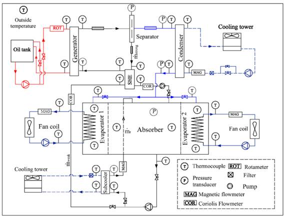
Aqueous LiBr solution inside the absorption chamber flows into two separate streams: a strong solution (solution poor in water or concentrated solution) coming from the generator, and a re-circulated solution. The strong solution is separated from the water vapor, which goes to the condenser, and directed to the absorber. A re-circulated solution is extracted from the bottom of the absorption chamber and pumped into the sub-cooler, where most of the absorption heat is rejected and then the sub-cooled solution is returned to the absorber. Two fan coils receive the external fluid circulating through each evaporator. The objective of placing two evaporators is to have a larger heat exchange area available and to guarantee the symmetry in the supply of vapor to the absorption vessel. Distribution problems in the refrigerant flow were detected; which will be discussed in following sections.
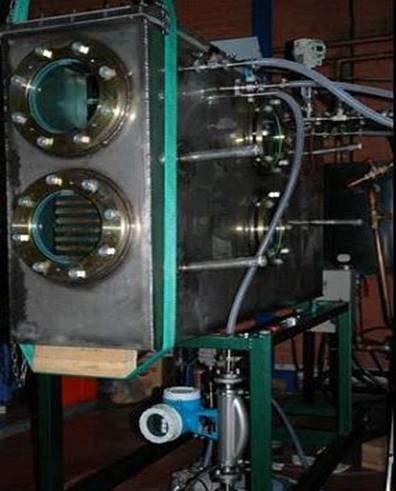
The experimental setup configuration and the experimental uncertainty analysis were described in detail in other publications (Gutiérrez et al., 2006; Gutiérrez et al., 2011). Figure 2 illustrates the experimental test facility.
Experimental test run
The data acquisition system is composed of two data-loggers, manufactured by Yokogawa, with 50 input ports available altogether, and a 24 V power supply. The oil flowmeter and the pressure transducers use the power supply to output an electric current of 4 to 20 mA. The input ports were read in intervals of 0.5 seconds.
The experimental procedure consists of periods of start-up, normal operation, and shut down of the machine. Start-up begins with the heating of the thermal oil from ambient temperature to the temperature set point t
set
while the oil is pumped to the generator. The solution pump is switched on and the weak solution flow rate
Table 1 Operating ranges of input variables
| Parameter | Working Range |
|---|---|
| Inlet oil temperature (tset) | 78.8 - 99 ºC |
| Weak solution mass flow rate ( |
169.6-363.5 kg/h |
| Recirculated solution mass flow rate ( |
261.8-1051.3 kg/h |
| Cooling water temperature, condenser | 18.9-30.8 ºC |
| Cooling water temperature, subcooler | 18.5-30.1 ºC |
| Chilled water temperature, evaporator 1 | 6.5-19.1 ºC |
| Chilled water temperature, evaporator 2 | 9.7-19.8 ºC |
| Refrigerant outlet temperature, condenser | 17-28 ºC |
| Refrigerant inlet temperature, evaporator 1 | 18.3-23.6 ºC |
| Refrigerant inlet temperature, evaporator 2 | 15.4-21.3 ºC |
| Refrigerant outlet pressure, condenser | 2.8-5.9 kPa |
| Low pressure | 0.7-1.9 kPa |
Figure 3 indicates the time period until stability is achieved (time elapsed until equilibrium). Some variables are plotted against time in order to show their evolution during a typical experiment. These variables are: inlet oil temperature,
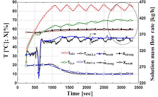
The stability of the working conditions is assured by selecting, from registered data, a period of time (20 min at least) in which temperatures, pressure and both
After this procedure, the recorded data corresponding to all sensors connected to the data loggers is averaged. Table 2 presents sensors used in the experimental test facility.
Table 2 Sensors used in the experimental test facility
| Instrument | Quantity | Range | Uncertainty |
|---|---|---|---|
| Thermocouple | 30 | 5 - 110 ºC | ±(0.2ºC - 0.6ºC) |
| Solution flow and density meter | 2 | 150-400 kg/h | ± 0.5% |
| Oil flowmeter | 1 | 1000-3600 l/h | ± 3.1% |
| Cooling water flowmeters | 2 | 1200-1500 kg/h | ± 1.1% |
| Recirculated solution flowmeters | 1 | 200-1000 kg/h | ± 1.3% |
| Fan coil flowmeters | 2 | 400-600 kg/h | ± 0.7% |
| Pressure sensors | 4 | 7-130 mbar | ±(1.8 - 3)% |
Experimental uncertainty analysis
A calibration process was carried out for all instruments described in Figure 1. Using the calibration functions for every sensor, systematic errors were reduced as much as possible. The remaining random uncertainty U for an experimental result R, which is a function of n independent parameters xi, is estimated, according to the Gauss algorithm, as:
The uncertainty of instruments is given in Table 2.
Relevant parameters
The performance parameters corresponding to each one of the operating conditions are obtained according the procedure explained in the previous section.
From measured values of inlet (i) and outlet (o) water temperatures t of both evaporators, cooling power is obtained from Eq. (2):
The heating power supplied to the generator was calculated as:
C corresponds specific heat capacity of a liquid and
The experimental COP was calculated as the quotient of (2) and (3).
In this work, the selection of variables involved in the obtaining of an ANN model is based on the proved dependency of the facility performance with external water circuit temperatures and the “overflow” of refrigerant in the evaporators (Gutiérrez et al., 2012). The overflow depends on the internal fluid temperatures of the liquid refrigerant at the condenser exit and the evaporators entries Tl,C, Tl,E1, Tl,E2, as well as the low pressure Plow and condenser exit pressure PC,o. Therefore, the input layer consists of 8 temperatures: The external fluid circuit temperatures in the generator, sub-cooler, condenser, and evaporators TG,set, Tcw,C, Tchw,E1
, Tchw,E2, respectively, and the above mentioned Tl,C, Tl,E1, Tl,E2. In addition, 2 mass flow rates, corresponding to weak and re-circulated solutions,
Another model was developed based on the principle of the accessibility of data in practical applications, with the intention that such model could be used as a black box. The variables selected for this scenario are the mean value of external fluid circuit temperatures: TG,set, Tcw,C, Tchw,E1 , Tchw,E2. Time is also included in this study in order to compare the simulated and experimental data in a transient experiment.
The output layer contains only one of the three variables: the generation power
Artificial neural networks model
Neurons are grouped into distinct layers (input, hidden and output layer) as well as interconnected according to a given architecture. The network function is determined largely by the connections between neurons. Normally, each connection between two neurons has a weight and bias coefficients attached to it. The standard network structure for an approximation function is the multiple-layer feed forward which has one or more hidden layers of sigmoid neurons followed by an output layer of linear neurons.
The linear output layer lets the network produce values outside the -1 to +1 range. The linear output layer function is used for forecasting the performance of the adiabatic absorption cycle (Hernandez et al. 2009b).
Learning algorithm
The learning algorithm is defined as a procedure that involves adjusting of the weights and biases, by minimizing an error function (usually a quadratic one) between the network output, for a given set of inputs, and the correct target. If smooth non-linearity is applied, the gradient of the error function can be computed by the classical back-propagation procedure (Natrick et al., 1998). In this work, the Levenberg-Marquardt algorithm optimization procedure -in the Matlab Neural Network Toolbox was used. This algorithm is an approximation of Newton’s method which was designed to approach second order training speed without having to compute the Hessian matrix (Martin et al., 1994). The root mean square error (RMSE) is calculated with the theoretical values and network predictions.
Database preparation
Steady states and transitory data were considered for the absorption system modelling by means of artificial neural networks. In order to characterize the system, 219 experimental points were obtained at different operating conditions (Table 1). These data was used to train and test the steady state and transient ANN models. For transient data base 1445 values were considered for a period of time.
In order to test the robustness and then the prediction ability of the models, the experimental database was split into the learning and testing database. Both transient and steady state experimental database were split into learning (80% of the data) and testing (20% of the data) with the objective of obtaining the best correlation between output target and output simulation and a good representation of the operating performance. With the learning database the optimal weights and biases are obtained and with the testing database the model is validated (Rumelhart et al., 1986). The model adequacy is obtained after testing the increment of neurons in the hidden layer. In this model, we avoided over-fitting by considering the comparison between the root mean square error (RMSE) obtained for both the learning database and the testing database (Hernández et al., 2009b).
The input layer consists of variables that the operator can control and/or that influence the equipment performance. In response to this, variables selected correspond to those listed in section 4. Input and output parameters were normalized for calculation from 0 to 1 (Khataee and Mirzajani, 2010).
Inverse artificial neural network
According to Hernández (2009); Labus et al. (2012); Hernández et al. (2012); Laidi and Hanin, (2013); Hernández (2013); Morales et al. (2015); the artificial neural network can be inverted to calculated a desired input parameter. In order to apply this inverse artificial neural network (ANNi), first it is necessary to have the ANN model. In this case, the multi-layer feed-forward (MLFF) is applied. If the hyperbolic tangent sigmoid transfer function is used in the hidden layer and the linear function is considered in the output layer then the output layer is:
Where:
In(k) = the inputs parameters
Wi = the weight between input and hidden layer
Wo = the weight between hidden and output layer
b1 = the bias in the hidden layer and
b2 = the bias in the output
S = the neurons number in the hidden layer
k = the parameters number in the input layer
Consequently, if the Equation 5 has more of one neuron in the hidden layer (S>1), then the inverse artificial neural network can be as following (Hernández, 2009a):
Where In(x) is the input parameter value to be calculated. Consequently, the Equation (6) can be solved using a method of optimization to obtain the desired input parameter. In this case, the Nelder-Mead simplex algorithm was applied.
In the case that the Equation 5 had only one neuron in the hidden layer then it can have an analytical solution (Hernández, 2009b).
Results and discussion
In this work, three neural network models were obtained from different configuration applied. First, steady state database was worked to obtain
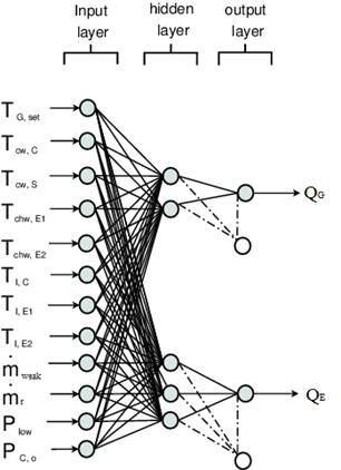
The input layers for these neural network models are also illustrated in this Figure 4. Table 3 shows the main characteristics of how neural network models work.
Table 3 Artificial neural networks models development in this work
| Φ | N° of neurons in the input layer |
N° neurons in the hidden layer |
Output layer |
R | Intercept | Slope |
|---|---|---|---|---|---|---|
| Model 1 (steady state) | 12 | 3 | QE | 0.9867 | 0.0056 | 0.9934 |
| Model 2 (steady state) | 12 | 2 | QG | 0.9879 | 0.0826 | 0.9826 |
| Model 3 (dynamic state) | 12 | 12 | QE | 0.9648 | 0.0738 | 0.9470 |
| Model 4 (dynamic state) | 12 | 16 | QG | 0.9790 | 0.1659 | 0.9653 |
The comparison of experimental
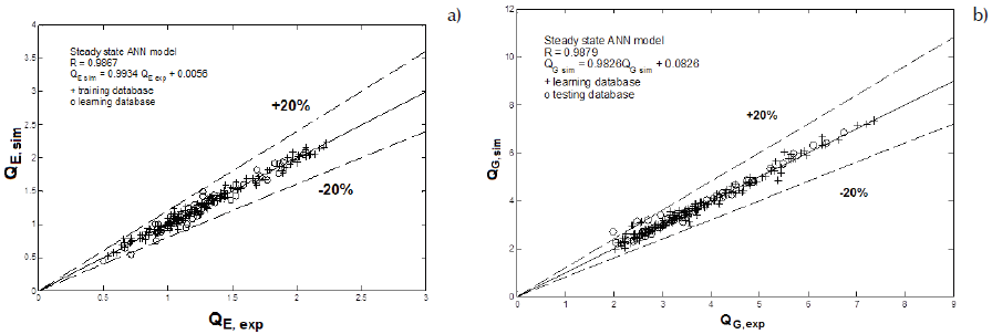
Figure 5 Experimental and simulated values of evaporator power
Regarding the results for transient data, the architecture of neural networks keeps the same input layer in this work using 12 operation variables. Experimental and simulated data of COP values were compared through a linear regression model in Figure 6. Again, satisfactory results were obtained with R>0.98 (
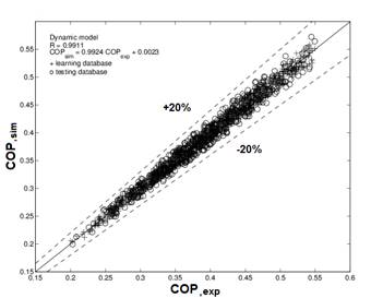
Figure 6 Experimental and simulated values corresponding to coefficient of performance using the dynamic database
The intercept a (-0.0011 < a < 0.0057) includes zero, and the slope b (0.9837 < b < 1.0010) includes 1. Consequently, the statistical significant correlation between experimental and simulated values at transient conditions was found.
The results corresponding to the additional model developed for transient data, which includes only the temperatures of external fluid circuits, are depicted in Figure 7a. In order to predict the coefficient performance 32 neurons in a hidden layer were necessary. The hyperbolic tangent sigmoid transfer function (
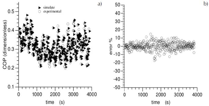
Figure 7a Experimental and simulated values of coefficient of performance COP vs. time using transient database Figure 7b. Relative error between simulated and experimental values of COP vs. time using transient database
Even though the dynamic behavior of a thermal device is complicated, the results obtained using an ANN analysis in a transient model were good. This tool allows us to determine a real-time coefficient of performance in order to make the necessary adjustments to optimize the operation of an absorption facility.
Optimum operating conditions using inverse neural network
According to the artificial neural network section presented in this work, it is possible to propose an online estimation strategy of the COP. The following steps were developed: First, it is possible to predict the coefficient of performance considering only external variables in the system. The temperatures at generator, condenser and temperatures corresponding to evaporator 1 and 2 were selected in this section. Second, training and validation of ANN model to predict the COP in transient state. The training procedure was carried out following the steps enlisted previously in the artificial neural network section. The ANN trained had 32 neurons in the hidden layer and
Experimental and simulated data of COP values were compared through a linear regression model in Figure 8 as:
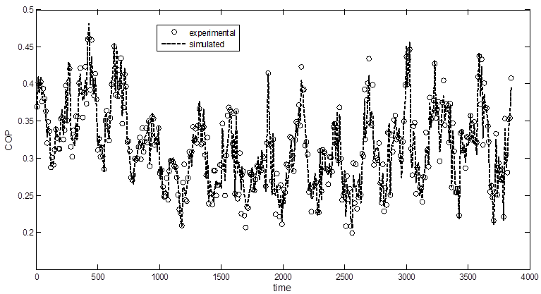
Finally, the artificial neural network inverse as optimization strategy. In addition to this, a strategy for optimizing the COP for the system has been developed. The selected strategy is the inverse neural network. With the aim of developing the artificial neural network to the experimental facility presented in this work, a test is carried out.
The direct neural network model is used to estimate the COP, based on the following operating conditions: TC = 21.93 °C, TS = 21.34 °C, TE1 = 15.77 °C, TE2 = 16.18 °C. The generator temperature is estimated as a function of time according to the following relationship:
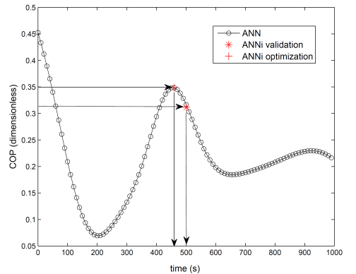
Equation (7) is used to reproduce the generator temperature TG versus time (t), keeping fixed operating conditions. Figure 9 shows the COP against time as the result of simulation of the direct neural network.
The inverse neural network is developed based on the following expression (Hernández, 2009b):
Where s is the number of hidden neurons and y i estimated as:
Weights and bias are obtained from direct neural network model.
It is possible to obtain the time when the system reaches the experimental point COP=0.3115. The numerical result obtained is t=503.8750 using the inverse neural network inverse methodology. The relative absolute percentage error calculated is 0.775% compared to time experimentally determined. The error is calculated as follows:
The computation time to solve the inverse neural network was 4.04 s.
However, the process could be reaching to a new stable state, or at least that indicates the simulation. In order to estimate the optimum COP, the inverse neural network strategy was applied for a second time. Assuming an optimal COP = 0.3485 (see Figure 8), keeping the operating conditions described above, the time in which the system reaches the optimum value is calculated. The calculated time with the artificial neural network is t = 476.5 s. The percentage error calculated was 3.59% compared to the time estimated using the direct neural network.
Conclusions
The application of artificial neural networks for modeling the performance of a particular adiabatic absorption facility has been developed in this work. Experimental results are included in steady and transient operations. Three models were obtained corresponding to cooling and generation capacities and coefficient of performance of the experimental system. These models were trained and validated with both steady and transient state experimental database. With the purpose of using a black-box model, an additional model was obtained using external circuit temperatures, with satisfactory results when compared in a transient experiment. Results demonstrated a good agreement between experimental and simulated values for all cases. The models obtained could be used to predict cycle performance or on-line estimation. Optimization of COP was carried out using an inverse neural network with satisfactory results. This method, applied to transient data, demonstrate to be a useful tool for control purposes.

