


 text new page (beta)
 English (pdf)
 Article in xml format
 Article references
 Send this article by e-mail
 Cited by SciELO
  Similars in
SciELO
Similars in
SciELO 
 Permalink
Introduction
The modeling chain in the evaluation of the climate change impact on hydrology generally includes climate simulations (in reference and future periods) from a global climate model (GCM) which are used to feed a hydrological model. Then, the simulated streamflow is compared in order to obtain the climate change signal between periods (Muerth et al., 2013). However, climate change impact studies are often based on GCM simulations dynamically downscaled by a regional climate model (RCM) instead of direct GCM simulations (e.g. Graham et al., 2007; Boé et al., 2009; Seiller and Anctil, 2014; Velázquez et al., 2015). In the dynamical downscaling approach, GCMs provide the boundary conditions to RCMs leading to high resolution physically-based climate simulations that improve the climate variables (Maraun et al., 2010). Nevertheless, GCM and RCM simulations have systematic biases (i.e., differences between the climate model simulations and the observations) that should be corrected in order to obtain consistent streamflow (Teutschbein et al., 2011).
Several studies have evaluated the advantages of the fine resolution provided by RCMs over GCMs in the representation of streamflow. For example, the study of Hay and Clark (2003) evaluated the performance of a RCM and a GCM (before and after bias correction) to reproduce observed streamflow in three large catchments in west U.S. Results show an advantage of the raw RCM simulations over the raw GCM outputs; thus, the former led to more realistic runoff simulations; however, both models showed a good performance after bias correction. On the other hand, Troin et al., (2015) compared the climate change signal (CSS) on hydrological indicators obtained with a given GCM and a coupled RCM-GCM over two snowmelt-driven Canadian basins. Results show similar direction and magnitude on the selected indicators, and authors claim that the use of GCM outputs can provide a good reproduction of the hydrological regime as RCMs do.
The scope of this study is the comparison of the climate change signal on hydrological indicators evaluated with a) simulations from the Canadian Global Model (CGC) dynamically downscaled by the Canadian Regional Climate Model (CRCM-CGC) and b) CGC simulations, over a Mexican basin. CRCM-CGC simulations, as well as other RCMs simulations, are included in the NARCCAP (North American Regional Climate Change Assessment Program) experiment (Mearns, et al., 2009) which provides high resolution climate scenarios for North America. Even if there are other experiments covering Mexico, NARCCAP provides easily available climate simulations in order to investigate climate change impact on water resources. The topic is interesting since the Mexican territory is partially covered by the CRCM-CGC (and other RCMs) domain (Figure 1). Therefore, if the climate change on hydrological indicators is similar either with the global or the regional climate simulations, the former could be used with confidence in the evaluation of the climate change impact on water resources in southern Mexico despite their lower resolution.
The manuscript is organized as follows: first, the methods and data are presented, including the study basin, the climate model simulations, the bias correction procedure and the hydrological model. Second, results of climate change signal on meteorological variables and streamflow are presented. Finally, conclusions close the manuscript.
Methods and data
Study catchment and observational dataset
The study catchment is the Tampaon River Basin located in east-central Mexico (Figure 2), which covers an area of 23 373 km2 (IMTA, 2016). The east part of the basin is located in the Sierra Madre Oriental mountain chain, which provides an orographic barrier to the Oceans’ precipitation that leads to a variety of climatic regions within the basin: the east region presents a tropical Savannah (Aw) and tropical monsoon (Am) climate types; the central region has a temperate dry winter hot summer (Cwa) climate type and the west region presents an arid cold steppe (BSk) climate type (Peel et al., 2007).
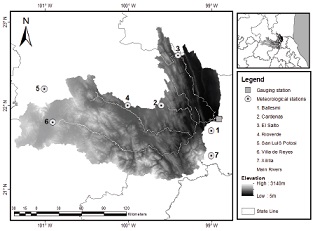
For this study, meteorological data from the stations depicted in Figure 2 were considered. The daily time series of precipitation and minimum and maximum temperature were obtained from the Climatologic Data Set (CLICOM, 2017) for the 1971-2000 period. The Tampaon River Basin has a mean annual temperature of 21.5⁰C and the area’s mean annual rainfall is 1080 mm. Table 1 shows the description of the hydro-meteorological stations considered in this study. The homogeneity of the precipitation data was evaluated with the Helmert test (e.g. Moreno et al., 2004). Results shows issues with station 24027; however, the station was retained, for the hydrological model efficiency was affected when such data were removed.
Table 1 Brief description of the hydro-meteorological stations used in this study
| Meteorological station | CLICOM ID | Lat (N) | Lon (W) | Elevation (m) | Available information period |
|---|---|---|---|---|---|
| Ballesmi | 24005 | 21.7° | 99.0° | 45 | 1961-2015 |
| Cardenas | 24006 | 22.0 | 99.6 | 1215 | 1929-2015 |
| El Salto | 24027 | 22.6 | 99.4 | 558 | 1954-2014 |
| Rioverde | 24114 | 22.0 | 100.0 | 991 | 1961-2015 |
| San Luis Potosí | 24069 | 22.2 | 101.0 | 1870 | 1949-2015 |
| Villa de Reyes | 24101 | 21.8 | 100.9 | 1820 | 1961-2015 |
| Xilitla | 24105 | 21.4 | 99.0 | 676 | 1964-2014 |
| El Pujal (gaugin station) | 26272 | 21.8 | 99.9 | 5 | 1953-2006 |
The discharge data were obtained from the National Database of Surface Water (IMTA, 2016) for the 1971-2000 period. These data come from the gauging station El Pujal (I.D. 26272), located downstream the Valles River. The gauging station drains the Tampaon River basin, whose farthest headwater is the Santa Maria River. This river flows west to east and its junction with the Verde River makes the start of the Tampaon River. From here, the Tampaon River flows to the northeast to join the Gallinas River and the Valles River (Velázquez et al., 2015). Figure 3 shows that the Tampaon River Basin presents two peak flows in July and September.
Climate simulations
The climate simulations were taken from the Canadian Regional Climate Model (CRCM) version 4.2.3 (De Elía and Côté, 2010), driven by a 5-member ensemble of the third generation Canadian Centre for Climate Modelling and Analysis Coupled Global Climate Model (CGC; Scinocca et al., 2008). In this investigation, the dynamically downscaled simulations (hereinafter referred to as CRCM-CGC, ∼ 45 km) were used along with the ensemble of climate simulations obtained from CGC (∼ 400km), under the SRES emission scenario A2. The IPCC emission scenarios are alternative images of the future considering different of demographic and socio-economic development and technological change. The increase of the global population and the technological change is more fragmented and slower for scenario A2 than in other scenarios. For instance, the projected change in mean global temperature is 3.4°C and 1.8°C for scenarios A2 and B1, respectively, for decade 2090-2099 compared to decade 1980-1990 (IPCC, 2010). Therefore, scenario A2 generally provides a larger CSS than other scenarios.
An estimation of the natural variability is given by the 5-member ensemble, which was obtained by repeating the climate change experiment using the climate model with changes in the initial conditions induced by small perturbations (Murphy et al., 2009). Periods 19712000 and 2046-2065 were selected for this study given the data availability for both climate models. Figure 4 shows the grid points considered in evaluating the climate change impact on the study basin for both the regional and the global climate model.
Bias correction procedure
The direct use of GCM or RCM climate simulations to feed a hydrological model generally leads to unrealistic streamflow due to systematic biases of the climate models (Teutschbein et al., 2011). Therefore, the correction of the time series of temperature (T) and precipitation (P) is necessary before being used in hydrological models.
The monthly bias between climate simulations and observations over the reference period (ref) is computed as equation 1.
where
The bias correction procedure used in this investigation was proposed by Mpelasoka and Chiew (2009), and the method had been largely applied to climate change impact studies (e.g. Chen, et al., 2013; Levison et al., 2014; Velázquez et al., 2015). In this bias correction method, a monthly transfer function between observations and climate simulations is found for the reference period for a given number of percentiles:
where T (corr) and P (corr) are the bias-corrected variables, the indexes correspond to percentile (q), monthly (m) and daily (d) time steps, raw climate simulations (sim) and observations (obs). In a second step, the transfer function is applied to climate simulations in future period under the hypothesis that the biases in future period will be the same than in reference period (Ho et al. 2012). For future period (fut), the corrected precipitation and temperature are obtained as:
For this study, fifty percentiles were calculated for each month. The bias correction method was performed with the meteorological observations of each meteorological station (see Table 1). Therefore, the climate models outputs were bias corrected and statistically downscaled for each meteorological station.
The hydrological model and the hydrological indicators
The model used in this study is GR4J, which is a conceptual lumped model that simulates streamflow at daily time step. GR4J uses mean daily precipitation (P) and potential evapotranspiration (PE) as input variables. PE was computed with the formulation proposed by Oudin et al. (2005), which is based in mean temperature and incoming solar radiation. A complete description of GR4J can be found in Perrin et al. (2003). The hydrological model was calibrated (1971-1985) and validated (1986-2000) over the study basin. The Nash-Sutcliffe Efficiency coefficient (NS; Nash and Sutcliffe, 1970) was used to compare the observed and simulated streamflow, and NS=1 corresponds to a perfect match between observed and simulated discharge. GR4J performs well as the NS obtained was 0.87 and 0.72 for the calibration and validation period, respectively.
Three hydrological indicators were used in this investigation:
The mean monthly streamflow (Qm), which is the mean of all of the daily values over a given monthly period.
The mean monthly high flow (Qmax), which is the mean of the maximum streamflow values for a given month.
The mean monthly low flow (Qmin), which is the mean of the minimum streamflow values for a given month.
The climate change signal (CCS) on hydrological indicators (I) was computed as the differences of simulated hydrological indicators from the reference
Results and discussion
Figure 5 shows the observed and simulated mean monthly precipitation and temperature over the Tampaon River Basin for the 1971-2000 period. The mean precipitation was computed with the Thiessen Polygon method, while the mean temperature was computed with the simple average. From Figures 5a and 5b, it can be seen that the maximum observed precipitation is presented in July and September, with a decrease in August due to the midsummer drought (Magaña et al., 1999). Table 2 shows the mean monthly bias in precipitation and temperature as computed with Eq. 1 and 2. The bias in precipitation is different for each climate model; for example, CGC (Figure 5a) overestimates precipitation in the dry season (November to May), thus, the bias ranges from 19.8 to 78.2 mm month-1, while in the wet season (June to October) the bias ranges from -3.8 to 42.5 mm month-1. On the other hand, CRCM-CGC (Figure 5b) overestimates precipitation in the dry season (from 10.1 to 50 mm month-1) and underestimates it in the wet season (from about -25.9 to -87.7 mm month-1).
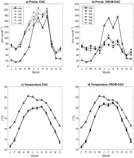
Figure 5 Observed and simulated mean monthly precipitation (upper panels) and mean monthly temperature (lower panels) for the 1971-2000 period over the study basin. The meteorological variables were obtained from CGC (left panels) and CRCM-CGC (right panels)
Table 2 Mean monthly bias in precipitation (bP) and temperature (bT) for the reference (1971-2000) period. The values are the average of the 5-member ensemble
| bP | bP | bT | bT | |||
|---|---|---|---|---|---|---|
| (CGC) | (CRCM-CGC) | (CGC) | (CRCM-CGC) | |||
| month | (mm month-1) | % | (mm month-1) | % | °C | °C |
| Jan. | 52.6 | 249.6 | 50.0 | 237.3 | -5.4 | -5.6 |
| Feb. | 45.4 | 309.7 | 46.1 | 314.0 | -5.1 | -5.6 |
| Mar. | 56.5 | 305.0 | 46.7 | 252.0 | -4.9 | -5.3 |
| Apr. | 74.9 | 176.5 | 21.3 | 50.1 | -4.2 | -4.0 |
| May. | 78.2 | 114.8 | -13.1 | -19.2 | -4.2 | -3.1 |
| Jun. | 25.9 | 18.0 | -62.4 | -43.4 | -3.3 | -2.1 |
| Jul. | 12.4 | 7.3 | -77.2 | -45.5 | -2.3 | -1.4 |
| Aug. | 42.5 | 31.3 | -59.7 | -44.0 | -1.9 | -0.8 |
| Sep. | 18.0 | 10.3 | -87.7 | -50.3 | -2.9 | -1.4 |
| Oct. | -3.8 | -4.8 | -25.9 | -32.6 | -3.8 | -2.9 |
| Nov. | 19.8 | 70.8 | 10.1 | 36.1 | -3.9 | -3.3 |
| Dec. | 35.0 | 134.4 | 23.5 | 90.2 | -4.7 | -4.4 |
Regarding the mean monthly temperature, Figures 5c and 5d show the observed annual cycle with a minimum on January (16.3°C) and a maximum on May (25.1°C). The bias in temperature is comparable in both climate models; that is, a general underestimation with values of about -5.5°C in January and from -0.8°C to -1.9°C in August. We can say that, despite the higher resolution, the regional climate model did not reduce the systematic bias of the global climate model simulations.
Figure 6 depicts the climate change signal on precipitation and temperature before and after bias correction. Regarding precipitation, the CCS for raw CGC ranges from -13 to -17%, and after bias correction, the CCS ranges from -13% to -19%. In addition, the CCS on precipitation for CRCM-CGC ranges from -24 to -27%, and from -26 to -29% before and after bias correction, respectively. These results show that bias correction changes the climate change signal. In that aspect, Muerth et al. (2013) claim that bias correction of climate simulations does not guarantee physical consistency and may affect the climate change signal to some extent.
Figure 6 Climate change signal on temperature and precipitation for the ensemble of climate simulations before (left panel) and after (right panel) bias correction
On the other hand, the climate change signal on temperature ranges from 2.3°C to 2.6°C for CGC, whereas for CRCM-CGC the CSS ranges from 2.7° to 2.9°. The CSS in temperature is not significantly changed after bias correction. Furthermore, results show that the climate change signal is larger for CRCM-CGC than for CGC for both meteorological variables.
In the next step, GR4J was fed with bias corrected climate simulations in order to obtain streamflow simulations in reference and future periods. Figures 7a and 7b show the hydrological annual cycle in the reference period as simulated with CGC and CRCM-CGC, respectively. Both climate simulations reproduce the observed annual cycle as well as the midsummer drought. Regarding future period (Figure 7c and 7d), both types of climate simulations lead to a decrease on streamflow, especially CRCM-CGC. Moreover, the annual cycle in future period is somewhat modified, since October’s streamflow is higher that September’s streamflow for some simulations (e.g. aey and aez).
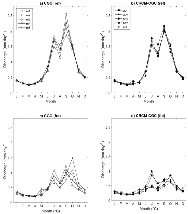
Figure 7 Mean monthly discharge as simulated with CGC (left panels) and CRCM-CGC (right panels) simulations for the reference (1971-2000; upper panels) and future (2046-2065; lower panels) periods
The simulated streamflow was used to compute the monthly hydrological indicators. Figure 8 shows the climate change signal on hydrological indicators evaluated for each member of the ensemble. The CCS was calculated over the same member; for example, the CCS for CGC member 1 was computed between member 1 in reference period and member 1 in future period. Such procedure leads to five CCS values for a given month and for a given hydrological indicator. Also, Figure 8 displays the CCS separated for the dry season (November to May) and for the wet season (June to October). The comparison of the median values in Figure 8 shows that, for all hydrological indicators, the CCS obtained with CRCM-CGC is larger than the CSS obtained with CGC. In addition, the decrease on hydrological indicators is larger for the wet season than for the dry season. For example, the median value of the CCS on Qm in the dry season (Figure 8a) is -21% and -28% for CGC and CRCM-CGC, respectively. Similarly, for the wet season (Figure 7b) the median CSS on Qm is -48% and -59% for CGC and CRCM-CGC, respectively. Comparing hydrological indicators, the most important decrease is estimated for Qmax in the wet season (Figure 7f), with values of -61% and -73% for CGC and CRCM-CGC, respectively.
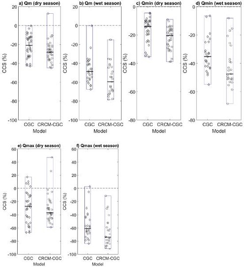
Figure 8 Climate change signal (CCS) on hydrological indicators obtained with CGC and CRCM-CGC for the study basin. The central mark in each box is the median CCS. The dry season ranges from November to May and the wet season from June to October
The Wilcoxon test (Wilcoxon, 1945) was used to compare the CCS on hydrological indicators obtained with CGC and CRCM-CGC. The null hypothesis is that two series of data are independent samples from identical distribution with equal medians (Wilks, 2006). Table 3 shows the result of the Wilcoxon test (p-value) performed to the series showed in Figure 8. In this table, it can be seen that the null hypothesis is rejected for all indicators, but for Qmax in the dry season (with a pvalue of 0.4737), for the CSS in precipitation is smaller in the dry season than in the wet season.
Table 3 Results of Wilcoxon test comparing the hydrological indicators obtained with CGC and CRCM-CGC. The p-value is shown and the shaded area indicates a rejection of the null hypothesis at significance level of 5%
| Hydrological Indicator | p-value |
|---|---|
| Qm (dry season) | 0.0458 |
| Qm (wet season) | 0.0137 |
| Qmin dry season | 0.0016 |
| Qmin wet season | 0.0123 |
| Qmax dry season | 0.4737 |
| Qmax wet season | 0.0283 |
The results of this study indicate that the CCS obtained with both types of climate simulations are different. Therefore, for the considered climate models, the choice of using the CGM simulations with or without the dynamical downscaling is an important aspect in the evaluation of the climate change impact on water resources.
Conclusions
This study compares the climate change signal on meteorological variables and hydrological indicators obtained with two 5-member ensembles of climate simulations for a reference (1971-2000) and a future (2046-2065) periods under the emission scenario A2: a) Canadian Global Climate Model (CGC) simulations dynamically downscaled by the Canadian Regional Climate Model (CRCM-CGC) and b) CGC simulations. The CRCM domain (as well as the domain of other climate models in the NARCCAP experiment) partially covers the Mexican territory; thus, the climate change impact on southern Mexicans basins cannot be evaluated with such simulations, losing the advantage of the higher resolution provided by the regional climate model. Therefore, this study assesses if the climate change signal obtained with the selected global and regional climate models is similar on direction and magnitude in one Mexican basin.
Results show that both types of climate simulations present biases in temperature and precipitation that do not allow their direct use to feed a hydrological model: CGC generally overestimates precipitation while CRCM-GCG underestimates precipitation in the wet season (June to October) and overestimates it in the dry season (November to May). On the other hand, both types of climate simulations generally underestimate temperature. Results also show that bias correction of climate simulations changes the climate change signal on meteorological variables, mainly in precipitation. Overall, CRCM-CGC leads to a larger climate change signal than CGC on meteorological variables.
The bias-corrected climate simulations were used to feed the hydrological model GR4J. The resulting streamflow simulations allowed the evaluation of the hydrological annual cycle. Results show that, in the reference period, both types of climate simulations lead to a correct representation of the hydrological regime, including the midsummer drought. Nevertheless, future streamflow simulations indicate a change on the hydrological regime, especially in the wet season.
The evaluation of the climate change signal on hydrological indicators shows that CRCM-CGC simulations yield to a larger decrease on streamflow than CGC simulations, especially for the wet season. Thus, the choice of using global or regional climate simulations is an important aspect in the assessment of the climate change impact on water resources for the study basin. Our results differ from the study of Troin et al., (2015) which did not find significant difference on the climate change signal on hydrological indicators evaluated with the global climate model and its dynamical downscaling over two Canadian basins. In that aspect, such Canadian basins have a hydrological regime which is highly sensitive to changes in temperature, for they are snow-melt driven basins which present maximum peak flows in spring. On the contrary, the Mexican basin in this study is rainfall-driven, so it is more sensitive to changes in precipitation, especially in the summer. In addition, the choice of the hydrological model has an influence on the simulation of streamflow (Velázquez et al., 2015), and future work should include several hydrological models to tackle this issue. Also, climate simulations obtained with the recent representative concentration pathways (van Vuuren et al., 2011) should be taken into account.

