


 text new page (beta)
 English (pdf)
 Article in xml format
 Article references
 Send this article by e-mail
 Cited by SciELO
  Similars in
SciELO
Similars in
SciELO 
 Permalink
Introduction
Lightweight flexible structures are increasingly being used in aerospace, automotive, construction, manufacturing, robotics, and other industries. Consequently, these structures are more sensitive to dynamic perturbations and the need for vibration control becomes crucial. Moreover, the requirement for simultaneous multimodal control increases because it is insufficient to just control the first dominant mode of light and flexible structures.
In the past few decades, active control of flexible structures using discrete or distributed actuators has been investigated to improve structural performances (Premount, 2002). These structures, with embedded or bonded sensors and actuators, are known as smart structures because their intrinsic ability to sense and control unwanted mechanical vibrations. Moreover, piezoelectric sensors and actuators have proven to be practical for structural control applications (Premount, 2011). These piezoelectric elements have been effectively applied in the closed loop control of different active structures including beams, shafts, plates, and trusses. Some of the attributes which have made piezoelectric actuators appealing for active control include the large useful bandwidth, the efficient conversion of electrical to mechanical energy, and the mechanical simplicity of the actuator with just a small extra weight added to the structures (Dosch et al., 1992).
Modal control is a preferred method in active control of flexible vibrating structures because it resembles the basic and intuitive notions of single degree of freedom systems. Modal control potential resides on mathematical matrix decoupling transformations (Inman, 2011). One of the simpler ways to reach modal active control is the pole placement method. In this control strategy, a designer has the flexibility to place the poles (eigenvalues) at the proper location for achieving the desired response.
Several researchers have applied a pole placement control scheme to suppress the unwanted vibration of flexible beam structures. Among them, Zhang and Li (2012) and Kumar and Khan (2007) have developed an adaptive pole placement technique in active vibration control. Zhang and Li (2012) studied the performance of adaptive pole placement control in a cantilevered beam. The robustness of the proposed controller was analyzed under various mechanical, electrical, thermal conditions. The investigation was done through simulation where a model was developed using the finite element method (FEM). Simulation results showed that the adaptive pole placement control is effective in controlling the vibration of the cantilever beam at various thermal conditions. Kumar and Khan (2007) proposed an adaptive pole placement controller for active vibration control of an inverted L structure. Experimental results have shown that the proposed controller is effective in suppressing the unwanted vibration caused by external force.
Pole placement method was applied with success by Bu et al. (2003) for control of the first dominant mode of a beam. A linear pole placement controller was designed by Sethi and Song (2005) for multimodal vibration suppression of a smart flexible beam by using piezoceramics as actuators and sensors. Experimental and numerical results demonstrated the effectiveness of multimodal vibration control of the first three modes of the structure.
The present work uses piezo-ceramic actuators and sensors for multimodal active vibration control of a flexible cantilevered beam, by using a single-input control, via feedback control. Control design of flexible structures depends on precise modeling of the system dynamics. Thus, finite element techniques are used to obtain a discrete model from the continuous beam dynamic model, leading to the equation of motion of the structure. This equation consists of a finite system of temporal second order coupled differential equations which, along with the sensor output equation, represent the discrete equation of motion of the smart structure. From the corresponding state space representation, modal control design of the smart structure is obtained by the pole allocation method within the feedback control approach.
Discrete smart beam model
Consider a Bernoulli-Euler type beam, with equilibrium equation given by
along with appropriate initial and boundary conditions. In Eq. (1), the parameters involved are
w |
= displacement response |
E |
= elastic modulus of beam material |
I |
= second moment of area of the beam cross section |
ρ |
= mass density of the beam material |
A |
= cross sectional area of the beam |
Q |
= external forces applied to the beam, including control forces |
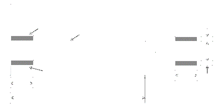
Now, consider a smart beam consisting of flexible aluminum cantilever beam with surface mounted piezoelectric sensor and actuator at the fixed end, as shown in Figure 1.
The external force input Q is taken as the sum of an external disturbance Q e, applied at the free end making the beam vibrate, plus a controlling force Q c. In this work Q e is considered null and free vibrations will only be produced by initial conditions
Finite element methods are used to obtain a discrete model of the beam equation with a finite number of degrees of freedom (DOF). By using 2-node Hermitian finite elements (2 structural DOF at each nodal point, displacement and slope), the equations of motion of the smart structure and the sensor output are given by Bandyopadhyay et al. (2007)
where
M
and
K
are the mass and stiffness n×n matrices, respectively, for a local composite piezoelectric element (beam plus piezo-patches) of length l
p,
q
is the vector of generalized displacements (displacements, w, and slopes, ∂w/∂x), and
with n i the i-th shape function, and
the mass per unit length and the flexural rigidity of the composite piezoelectric beam element, respectively. Note that the mass and stiffness matrices M and K in the system (3) can be varied by changing the location of the piezo-patches on the beam and by varying the number of regular and piezoelectric beam elements. A regular beam element can be obtained by just setting t p = I p = 0 in Equations (5).
The sensor output is the sensor output voltage and is computed from
where
n
is the shape functions vector, G
c is the signal conditioning gain,
where
The algebraic eigenvalue problem
Control forces are normally designed to modify the system characteristics so as to produce a desired response. The object is to coerce the response to certain perturbations to come close to zero asymptotically. The behavior of a linear dynamical system is governed by its eigenvalues. In fact, the response approaches zero asymptotically if the real part of all the system eigenvalues are negative. The goal of feedback control is to adjust the open-loop system so that all the eigenvalues of the closed-loop system acquires negative real part. This is equivalent to controlling the system modes (modal control). Consequently, knowledge of the open-loop eigenvalues of the system is critical.
To establish the open-loop eigenvalue problem, the open-loop system is considered by setting Q e= Q c= 0 in Eq. (3)
In control theory is more convenient to work with the state equations. Hence, by introducing the 2n-dimensional state vector
the state equations can be cast in compact form
where
is the 2n×2n coefficient matrix. The solution of Eq. (10) is
with λ a scalar and u a constant vector. Substituting Eq. (12) into Eq. (10), the algebraic eigenvalue problem is obtained
Recalling that A is 2n×2n matrix, the eigenvalue problem can be stated as
where λ i and u i are the eigenvalues and eigenvectors of A , respectively. Furthermore, the adjoint eigenvalue problem associated with A T is defined by
Equations (15) can also be written in the form
Since their position relative to A , u i are called right eigenvectors of A and v j are known as left eigenvectors of A.
It is convenient to normalize the eigenvectors, such that the eigenvectors become biorthonormal
with δ ij the Kronecker delta.
Feedback control
The state equations and output equations in matrix form are
and
respectively. For feedback control, the input u(t) takes into consideration the actual response of the system. When u(t) depends on the state of the system, then this case is called state feedback control, and
where G is known as the feedback gain matrix, or the control gain matrix.
Introducing Eq. (20) into Eq. (18) leads to
Control stability is governed by the eigenvalues of A-BG . The eigenvalues of A are known as open-loop eigenvalues (open-loop poles) and the eigenvalues of A-BG are known as closed-loop eigenvalues (closed-loop poles). Then, the object of linear feedback control is to ensure that the closed-loop poles lie in the left half plane of the complex plane, thus guaranteeing asymptotic stability.
From Eq. (21), the closed-loop poles depend on the control gains, that is, on the entries of the control gain matrix G . Two of the most widely used methods for computing control gains are pole allocation and optimal control. In this work we concentrate on pole allocation method.
Pole allocation method
As mentioned, the object of linear feedback control is to place the closed-loop poles on the left half of the complex plane of the eigenvalues so as to ensure asymptotic stability of the closed-loop system. One method consists of prescribing first the closed-loop poles associated with the modes to be controlled and then computing the control gains required to produce these poles. The algorithm for producing the control gains is known as pole placement.
The complexity of the procedure depends on the number of inputs. The number of inputs affects the details of the procedure in such a way that there are different algorithms corresponding to different cases. In this work we concentrate on the case of single-input control, and the following algorithm, originally proposed by Porter and Crossley (1972), was taken from the book by Meirovitch (1980).
For the case of a single input, the state equation (18) takes the form
where b is a constant 2n-vector and u(t) is the single control input. The open-loop eigensolution consists of the eigenvalues λ i , and the right and left eigenvectors, u i and v i , i = 1, 2,…, 2n. The two sets of eigenvectors are assumed to be normalized, so that they satisfy the biorthonormality relations (17).
We consider control of m modes and assume that the control force has the form
where g j ( j= 1, 2, …, m) are the modal control gains. Inserting Eq. (23) into Eq. (22), the closed-loop equation is
where
and it is noted that
so that the control given by Eq. (23) is such that the closed-loop eigenvalues and eigenvectors corresponding to the uncontrolled modes are equal to the open-loop eigenvalues and eigenvectors, respectively. It can be verified that the same is not true for the eigenvalues and eigenvectors associated with the controlled modes, j = 1, 2,…, m.
Next, we denote the closed-loop eigenvalues and right eigenvectors of C associated with the controlled modes by ρ j and w j ( j = 1, 2,…, m), respectively. But, because the open-loop right eigenvectors are linearly independent, they can be used as a basis for a 2n-vector space, so that the closed-loop eigenvectors can be expanded in terms of the open-loop eigenvectors as follows
Recalling the biorthonormality relation (17), the closedloop eigenvalue problem can be written in the form
Moreover, letting
Eqns. (28) become
which are equivalent to 2n×m scalar equations
Solution of the above equations leads to the gains
Clearly, for g j to exist, it must be p j ≠0. If any one of the p j is zero, then the associated mode is not controllable. Finally, the control law is obtained by inserting Eq. (32) into Eq. (23).
Numerical experiments
The smart beam was divided into 4 finite elements: one piezoelectric beam element (element 1 in Figure 2), and three regular beam elements (elements 2 to 4 in Figure 2). The geometric and material properties of the smart beam components (Al beam, sensor, and actuator) are given in Table 1. The beam has one end fixed and one end free. The discrete model has 8 degrees of freedom (dof´s), 4 dof´s associated with transverse displacements, and 4 dof´s associated with slopes.
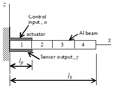
Table 1 Geometric and material properties of beam and piezoelectrics
| Geometric and material parameters | Aluminum beam | Piezoelectric PZT actuator/sensor |
|---|---|---|
| Length | l b = 0.3 m | l p = 0.075 m |
| Width | b = 0.03 m | b = 0.03 m |
| Thickness | t b = 0.5 mm | t a = t s = 0.35 mm |
| Density | ρ b = 2700 Kg/m3 | ρ p = 7700 Kg/m3 |
| Elastic Modulus | E b = 70 GPa | E p = 193 GPa |
| PZT strain constant | d 31 = 125×10-12 m/V | |
| PZT stress constant | g 31 = 10.5×10⁻³ Vm/N |
The physical properties of the flexible beam and the piezoelectric elements are given in Table 1. A Maple© code was written to implement the numerical model and the control algorithm. The open-loop eigenvalues of matrix A calculated by solving the eigenvalue problem (13) are shown in Table 2. If the first three lowest modes are to be controlled, corresponding to the eigenvalues λ 1,2 = ± 311.09i , λ 3,4 = ± 1951.73i , and λ 5,6 = ± 5500.95i , then the closed-loop poles are obtained by placing the first three poles by an amount -2.0 into the negative real part, which corresponds to damping ratios of 0.64, 0.10 and 0.04, respectively. The closed-loop poles are shown in Table 3. It is necessary to mention that two additional values of pole displacement were considered, -1.0 and -3.0; however, according to numerical results, and endorsed by the justification below, the displacement of -2.0 was selected to run the experiments. Accordingly, it is essential to point out that pole placement is arbitrary as long as a necessary and sufficient condition is satisfied. This condition is that the system be completely state controllable. Thus, in order to test state controllability, the 2n×2nr controllability matrix C is considered
Table 2 Open-loop eigenvalues
| Eigenvalues | |
|---|---|
| λ 1,2 | ± 311.09 i |
| λ 3,4 | ± 1951.73 i |
| λ 5,6 | ± 5500.95 i |
| λ 7,8 | ± 10852.67 i |
| λ 9,10 | ± 20184.73 i |
| λ 11,12 | ± 32415.37 i |
| λ 13,14 | ± 51390.81 i |
| λ 15,16 | ±84321.53 i |
Table 3 Closed-loop poles
| Eigenvalues | Damping rat | |
|---|---|---|
| ρ 1,2 | -2.0 ± 311.09 i | 0.64 |
| ρ 3,4 | -2.0 ± 1951.73 i | 0.10 |
| ρ 5,6 | -2.0 ± 5500.95 i | 0.04 |
| ρ 7,8 | ± 10852.67 i | - |
| ρ 9,10 | ± 20184.73 i | - |
| ρ 11,12 | ± 32415.37 i | - |
| ρ 13,14 | ± 51390.81 i | - |
| ρ 15,16 | ±84321.53 i | - |
where n is the number of degrees of freedom, and r is the number of displaced poles. Then, the system is completely state controllable if C has rank n. For the case under study, n = 8, r = 6, and it is verified that C is a 16×96 matrix with 8 linearly independent columns which implies that rank(C) = 8. Consequently, pole allocation can be arbitrarily done. However, there are some guidelines for choosing the locations of desired closedloop poles: If the closed-loop poles are chosen far away from the open-loop poles, the system will demand high control effort from the actuator; if the closed-loop poles are very negative, the system will be fast reacting, the signals in the system become very large, with the result that the system may become nonlinear; this should be avoided.
Using Eq. (32), the calculated gains corresponding to the located poles have the values
The control input u(t) is calculated by using Eqs. (20) or (23), where the gain matrix is given by
Accordingly, the closed-loop equation (Eq. (24)) can be stated, where C is given by Eq. (25). It is worth noting that vector b in (25) is calculated from Eq. (29), whereas p k is calculated from the expression
Finally, in order to obtain the transient response, the transition matrix approach is used. Thus, taking into consideration that the closed-loop equation
is subjected to the initial condition
then, the solution of the closed-loop equation is
where Φ(t) is the transition matrix given as the series
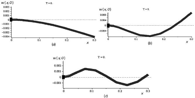
Three cases are considered in which the initial conditions are such that they incite free vibrations of the beam according to the first, second, and third vibration mode, respectively. The configurations of the three sets of initial conditions for the smart beam are represented in Figures 3a and c, with zero initial velocity. It is noted in these figures that the position of the piezo-actuator remained constant for the three experiments.
Discussion and analysis of results
In order to select the appropriated closed-loop pole allocation into the left half of the complex plane, three values of pole displacement were considered for first vibration mode only, -1.0, -2.0 and -3.0. According to numerical results, which are not showed here for space limitations, when the closed-loop poles are displaced by an amount of -1.0, the system is slow reacting with the vibration amplitude decaying to zero after 4 seconds, double the time than for -2.0, while the amplitude of the control vector reduces to one half. On the other hand, when closed-loop-poles are displaced by a quantity of -3.0, the system is fast reacting with vibration vanishing after 1 second, but the amplitude of the control vector is raised more than two thirds of the amplitude corresponding to -2.0 displacement. This behavior was expected according to the effects mentioned in the guidelines for choosing the locations of desired closed-loop poles cited in the previous section. Consequently, closed-loop pole displacement of -2.0 was considered to be more representative for numerical simulation purposes.
Figure 4a shows the transient response of the free end of the beam when the first vibration mode is excited and a unit voltage is applied to the actuator, while Figure 4b displays the control vector. It is observed that when the poles are displaced by an amount of -2.0 the vibration vanishes after 2 seconds. Similarly, Figures 5a and b show the response of the free end of the beam and the control vector, respectively, when the second mode is excited and a unit voltage is applied to the actuator. Again, the vibration reduces drastically after 2 seconds, however it is noted that some low amplitude vibration remains beyond this time; in addition, it is observed that the magnitude of the control vector is larger for the second mode than for the first mode. Finally, Figures 6a and b illustrate the response of the free end of the beam and the control vector, in that order, when the third vibration mode is excited; a similar behavior is observed in the third mode as in the second mode, where some small amount of vibration remains after 2 seconds, while the magnitude of the control vector is not as larger as in the second mode.
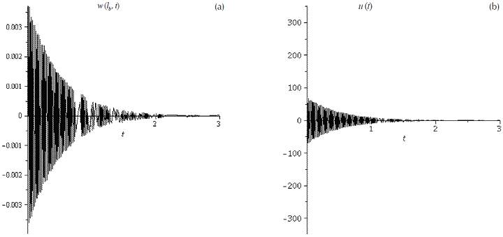
Figure 4 a) Transient response of the free end (x= l b ) of the beam, first mode, b) control vector applied to the actuator
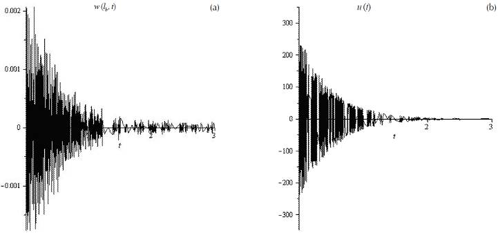
Figure 5 a) Transient response of the free end (x= l b ) of the beam, second mode, b) control vector applied to the actuator

Figure 6 a) Transient response of the free end (x= l b ) of the beam, third mode, b) control vector applied to the actuator
The observed behavior of the flexible smart beam can be explained by noting that the actuator remains at the fixed end for the three excited vibration modes, see Figure 2. This position corresponds to the highest strain along the beam for mode one, see Figure 3a, while the corresponding highest strain position for the beam in mode two is located at the middle of the span of the beam, Figure 3b, and for the beam in mode three there are two highest strain positions located at one-third and two-third of the beam length, Figure 3c. Consequently, vibration attenuation is more effective in mode one since the actuator operates straight at the zone with the highest strain, influencing more directly in beam bending with a small control effort. On the other hand, for vibration in mode two and three, the higher strains positions do not coincide with the position of the actuator. Therefore, the actuator works at a zone without a high strain, manipulating less indirectly beam bending with a higher control force.
Conclusions
The pole allocation method was applied in feedback vibration control of a smart continuous cantilevered beam structure. Finite elements techniques were used to obtain the discrete equation of motion, and from the related state space representation, control gains were obtained by the pole placement method for the appropriate modal control. Solving the algebraic eigenvalue problem was a crucial part of the analysis. The results obtained show that control of the first three modes of vibration was successfully accomplished with a single input, by using a piezo-actuator placed in a position which remained constant. This is more than evident for the first mode where the amplitude of the vibration completely decreases to cero after two seconds; however, for the second and third modes, some very low amplitude vibration remains in the flexible beam, while the control forces are larger for the second and third modes than for the first mode. This is a consequence of the actuator placed at the longitudinal position of the beam with the highest strain (fixed end) for mode one, while the corresponding highest strain position for the beam in mode two is located at the middle of the span of the beam, and for the beam in mode three there are two highest strain positions located at one-third and two-third of the beam length. Of course, if vibration in modes two and three is to be completely controlled, placing additional actuators along the beam is needed but at higher expenses considering multiple input-multiple output systems.

