


 nueva página del texto (beta)
 Inglés (pdf)
 Artículo en XML
 Referencias del artículo
 Enviar artículo por email
 Citado por SciELO
  Similares en
SciELO
Similares en
SciELO 
 Permalink
Introduction
Gas turbines are very sophisticated and costly systems that have been used in the past decades for different industrial applications due to the capacity to produce great amount of energy and because of their high efficiencies (Boyce, 2006). Since faults and gradual deterioration affect extremely the reliability and maintenance costs, gas turbines need advanced condition based maintenance and condition monitoring systems to ensure a correct operation (Rao, 1996). The success of these systems depends on the enhancement of monitoring software, the degree to which engine critical elements are covered and the accuracy of diagnostic decisions. Nowadays, different gas turbine diagnostic algorithms are developed to identify as accurate as possible faults conditions of major components (e.g., compressor, combustion chamber and turbine). Gradual deterioration and abrupt faults (Meher et al., 2001) and sensor faults (Kobayashi and Simon, 2008) can be detected as well. This is achieved by measuring principal gas path parameters such as pressure, temperature, rotation speed, fuel rate, etc.
In order to contribute to the diagnostic process improvement, the aim of this paper is to perform a gas turbine diagnostic algorithm testing. In previous works (Cisneros et al., 2015; Felipe et al., 2015), only preliminary results were obtained and some algorithms were tested separately. However, in gas turbine monitoring systems, an integrated approach is necessary to have more exact and reliable results. For this reason, the present investigation proposes a methodology comprising three unified stages. In the first stage, the gas turbine data is obtained using the software ProDiMES which works with no-fault conditions, faults and degradation mechanisms. This software is used because not only simulates a complete turbofan engine fleet based on a high-fidelity thermodynamic model but also allows evaluating gas turbine diagnostic algorithms (Simon et al., 2008 and 2013). To simulate real behavior for each engine, the software assigns unique deterioration profiles, noise levels and operation modes.
In the second stage, a baseline model testing is carried out to improve the healthy engine performance approximation. Besides, baseline models allow computing deviations, which are indicators of an engine’s state (Loboda et al., 2004). Three variations are proposed using simulated data with no-fault scenarios through ProDiMES and the model with the lowest total error is selected for the fault recognition stage. A baseline model can be developed based on a thermodynamic model or artificial neural networks (Loboda and Feldshteyn, 2010). The first option needs complex algorithms while the second one requires considerable execution time for training. Consequently, the present paper uses a polynomial function to ease the diagnostic algorithm. The least squares method is employed to calculate model coefficients determining the baseline model.
In the third stage, the baseline model selected is used as a basis to perform the fault recognition. With the intention of extracting the diagnosis information from raw data, it is necessary to use deviations calculated using actual measurements generated by simulating fault scenarios and healthy engine values. Three steps are proposed to compute deviations:
Initial deviation computation using a general model,
Creation of individual models and
Final deviation computation using individual models.
With these final deviations, normalized vectors (also called patterns), can be obtained to form a diagnostic space and perform the fault recognition. Gas turbine fault diagnostics, particularly the gas path fault identification, is based on pattern recognition techniques such as Radial Basis Network (Loboda et al., 2010), Probabilistic Neural Network (Tsalavoutas et al., 2000), Bayesian Network (Romessis and Mathioudakis, 2004) and Multi-Layer Perceptron (MLP) (Roemer and Kacprzynski, 2000; Volponi et al., 2000; Sampath and Singh, 2004). The latter technique has been applied widely in the past years and has shown that is it not inferior to other methods (Loboda et al., 2010). Therefore, this work uses the MLP to calculate the probability of correct diagnosis. The methodology utilized is implemented in Matlab. Its neural network toolbox (Beale et al., 2014) assists in an efficient development of the algorithm.
The paper is organized as follows. Section 2 gives the description of the methodology proposed. Section 3 describes the pattern recognition method used. Section 4 presents the results obtained for the baseline model testing and the gas turbine fault recognition.
Methodology proposed for gas turbine diagnostics
The methodology proposed (Figure 1) includes the following main stages:
Gas turbine data simulation using the software ProDiMES (Propulsion Diagnostic Method Evaluation Strategy),
Baseline model testing to enhance the healthy engine performance approximation and
Gas turbine fault recognition and the calculation of diagnosis accuracy. The stages are described in the below subsections.

Gas turbine data simulation using the software ProDiMES
Most of the real gas turbine faults are not so severe or rarely occur in practice to be sufficient for a complete fault description. Also, physical experimentation is not a feasible option because of the very high costs. Instead, mathematical models are applied (Saravanamuttoo and MacIsaac, 1983). This work uses the software ProDiMES as a tool to simulate a fleet of engines and study the algorithms for gas turbine fault diagnostics. ProDiMES was developed by the NASA Glenn Research Center originally intended for benchmarking international gas path diagnostic methods (Simon et al., 2008 and 2013).
ProDiMES includes an Engine Fleet Simulation (EFS) that generates simulated measurement parameter histories for each engine of the fleet. To simulate real engine behavior, it works with a deterioration profile, noise level and operation mode (takeoff and cruise) unique for each engine. The EFS is implemented in Matlab and consists of a Graphical User Interface (GUI), a Case Generator and a C-MAPPS Steady State engine model (Simon, 2010). Each element is described below.
Graphical User Interface (GUI)
In the Graphical User Interface (GUI), the user can control the type and the number of faults occurring in the engine fleet. The maximal number of possible simulated faults is 18 plus a no-fault case. Table 1 shows these fault cases and their magnitudes, within which the faults are distributed uniformly. Module faults (ID 1-5) corresponding to Fan, LPC, HPC, HPT and LPT are simulated by adjusting at the same time efficiency η and flow capacity γ parameters. Actuator faults (ID 6-7) corresponding to VSV and VBV result from a mis-scheduling between the commanded and current actuator position. There are also 11 different sensor faults (ID 8-18) whose magnitudes are in units of average measurement noise standard deviation σ. It is important to mention that in EFS, each individual engine only experiences a single fault type. Other aspects to consider are: the number of flights to generate the output data (the maximal number is 5000 flights per engine); the fault evolution type (abrupt or rapid); the flight of fault initiation (the 11th flight is the lowest value) and the sensor noise (on or off).
Table 1 Simulated fault cases (Simon, 2010)

*LPC=Low Pressure Compressor, HPC=High Pressure Compressor, HPT=High Pressure Turbine, LPT=Low Pressure Turbine, VSV= Variable Stator Vane, VBV=Variable Bleed Valve
The EFS works with eleven sensed variables. The seven measured variables shown in Table 2 are available for monitoring and are represented by a vector Y. Table 3 shows four measured variables used as operating conditions represented by a vector U. All the variables correspond to an engine standard measurement system.


Case generator
The case generator produces parameter histories after the user has selected the number and type of faults in the GUI stage. One important characteristic is the random generation of unique faults, degradation profiles and operating history for each engine in the fleet. This also includes the following assignations: the date when the collection of the engine data starts, the city pairs for the takeoffs of the engine, the ambient pressure, the atmospheric temperature, the Mach number and power setting parameters for takeoff and cruise. The level and rate of gradual performance deterioration for each engine are also considered by the Case Generator. They emulate the degradation that an aircraft engine experiences during its lifetime due to different effects such as fouling, erosion, and corrosion of blades and vanes. The gradual deterioration is not considered a fault and its development is much slower than the produced by faults.
C-MAPSS Steady-State engine model
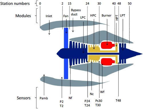
The Commercial Modular Aero-Propulsion System Simulation (C-MAPSS) Steady State is a high-bypass turbofan engine model created for diagnostics research (Simon, 2010). This model is run inside the EFS and receives the outputs from the Case Generator to produce the simulated measurement parameter histories for each engine, at takeoff and cruise of each flight. C-MAPSS works with two spool speeds (fan and core speed). Figure 2 shows the station numbers, the modules and the simulated sensor variables of the C-MAPSS Steady-State model.
Baseline model testing
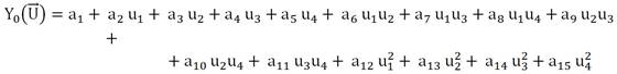
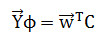
In order to know the current gas turbine condition by means of measured gas path variables, it is necessary to describe correctly its healthy state. According to Loboda et al., (2004), a good approximation of healthy engine performance, also called baseline model, can be given by complete second order polynomials. Also, polynomials have shown to be better than other techniques (Loboda and Feldshteyn, 2010). Considering one monitored gas path variable Y as function of four operating condition arguments U, the baseline model can be expressed as
 (1)
(1)
where a1, …, a15, are the model coefficients calculated using the least squares method for all monitored variables.
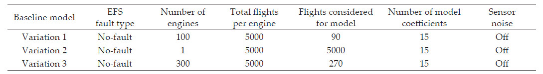
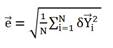
To find an adequate baseline model, three model variations are proposed by simulating no-fault cases (healthy engine scenarios) through EFS for cruise operation point. These variations are specified in Table 4 containing their principal characteristics and are briefly described as follows. Variation 1 is created using 100 engines and 5000 flights per engine, however, only the first 90 flights are taken into consideration to form the model because the deterioration is not so great in that interval. Variation 2 works with 1 engine and 5000 flights. Variation 3 simulates 300 engines and 5000 flights per engine but, only 270 flights are considered for model creation. For all variations, the number of model coefficients is k=15 and sensor noise is not considered. The criterion to select the best variation is based on the lowest total model error. First, an error for one monitored variable δY is calculated as
 (2)
(2)
where Y* and Y0 are measured and baseline model values respectively. Then, the total error
 (3)
(3)
After finding the model variation with the lowest
Gas turbine fault recognition
Deviation computation
Due to the variation of gas turbine operation conditions, absolute gas path monitored parameters change as well. Since these changes are greater than the produced by faults, the latter remain hidden. Therefore, a diagnostic process requires an important step of deviation computation to reveal deterioration and faults effects (Loboda et al., 2004). Three steps are proposed to calculate deviations needed for the gas turbine diagnostic algorithm:
Initial deviation calculation using a general model,
Creation of individual models,
Final deviation calculation using individual models.
1. Initial deviations using a general model. After selecting the variation model with the lowest error, the (k×m)-matrix C of model coefficients is used to form the general baseline model. It can be expressed as
 (4)
(4)
where
 (5)
(5)
Using the mean of these deviation vectors for the first n=10 simulated flights per engine (before the fault initiation) and considering one engine, we have
 (6)
(6)
where
2. Creation of individual models. As mentioned before, the Case Generator randomly assigns a unique operating history and deterioration profile to each engine in the fleet. However, the general model (4) does not contain these individualities. For this reason, individual models are needed before calculating the final deviations. Considering one flight and one engine, an individual model vector for all monitored variables is given by
 (7)
(7)
where
3. Final deviation calculation using individual models. Using individual baseline values Yρ for a monitored variable, we obtain
 (8)
(8)
where δYρ is a final deviation. These deviations are the base of fault class formation.
Fault class formation
With the intention of having a homogeneous diagnostic process, deviations (8) are normalized as follows
 (9)
(9)
where σY is a mean deviation error. One vector
 (10)
(10)
Thus,
 (11)
(11)
In ProDiMES, each fault class is constructed from patterns with the change of only one fault parameter (singular fault class).
Training and validation
In a pattern recognition process, the data can be separated into two parts: training and validation sets. Both sets are described shortly below and summarized in Table 5. The training set ZT unites patterns of all classes and is employed to train the method under analysis. It is formed by simulating all the 19 fault cases available in ProDiMES for better verification of the diagnostic algorithm (18 faults + 1 no-fault case), a determined number of engines per class and flights per engine for cruise operating point. The flight fault initiation selected is 11 with the option “fixed”, this means that the first 10 flights will not experience any fault. The fault evolution rate is selected as “rapid”. Since accuracy of fault classes’ description depends on the number of simulated patterns, 100 engines per class and 50 total flights per engine are considered. However, the number of flights per engine for rapid fault evolution is 34. For this reason, 3400 patterns per class are employed. Thus, the total size of the training set is 64600 patterns (19 fault cases × 100 engines × 34 flights).
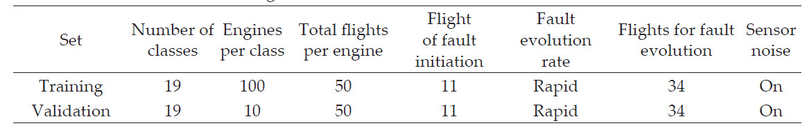
The validation set ZV is created to verify that the network can generalize the fault classes correctly. It is formed in the same manner as the training set ZT; however, its size is ten times smaller because it works with 340 patterns per class. Therefore, the total size of the validation set is 6460 patterns (19 fault cases × 10 engines × 34 flights). Every pattern in the validation set belongs to a known class.
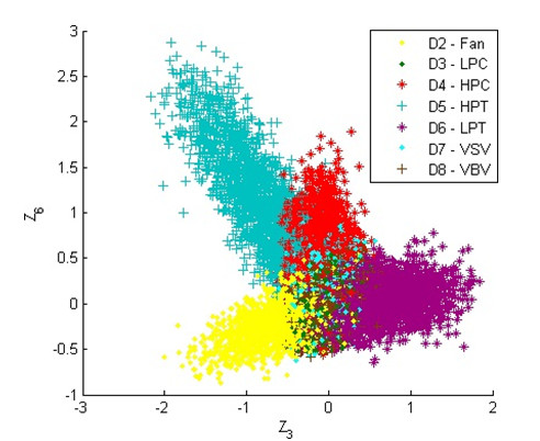
Figures 3, 4 and 5 exemplify the fault class formation using patterns of Z T in the space of two normalized deviations: Figure 3 shows class 1 (no fault) and class 4 (HPC fault); Figure 4 shows faults 2-8 including component and actuator faults; Figure 5 shows sensor faults 10-14.


Diagnosis accuracy
The fault recognition method selected classifies each pattern of the set ZV, producing the diagnosis d1. Comparing d1 with a known class Dn for all validation set patterns, a confusion matrix is generated. Its diagonal is formed by correct pattern classification probabilities per class. A mean number
Fault recognition method
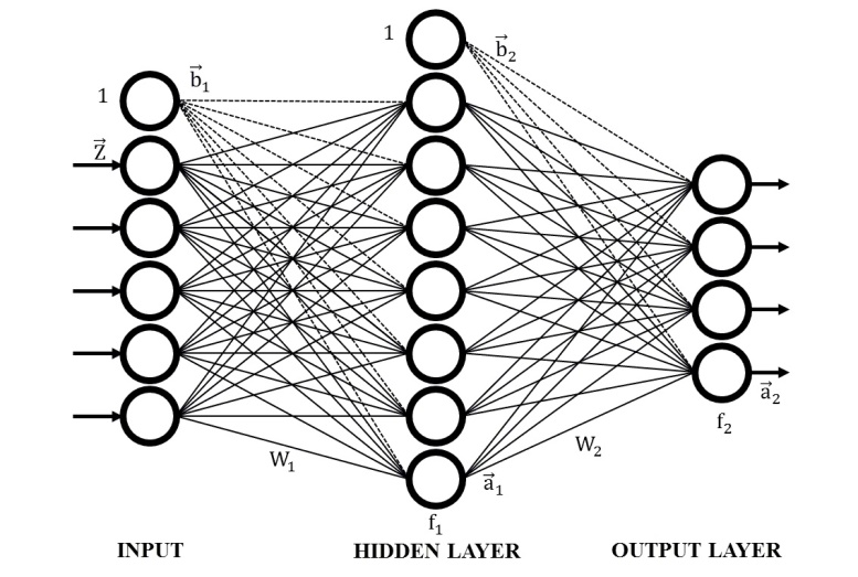
The fault recognition method chosen for this work is the Multi-Layer Perceptron (MLP). The MLP is an artificial neural network intended for classification problems. It uses a back-propagation algorithm that propagates a signal for a given input vector, producing an output and adapting unknown coefficients based on the error between a target and the network output. Figure 6 shows the general structure of the MLP. The input for each hidden layer neuron is given by the sum of an input vector
Diagnostic algorithm results
Errors of model variations
As shown in (Cisneros et al., 2015), Variations 1 and 3 contain displacements in their plots of errors δY at certain intervals due to the influence of each engine. This situation was addressed in Subsection deviation computation to correct individualities of all engines. Figure 7 shows the errors of Variation 2 for 5000 flights and one monitored variable. Here, the engine degradation effect is observable through all flights. Each engine in the fleet experiences this inevitable situation.

The total error

Fault diagnosis accuracy
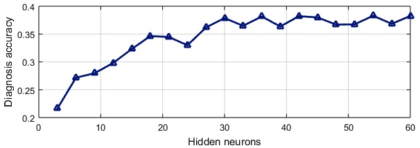
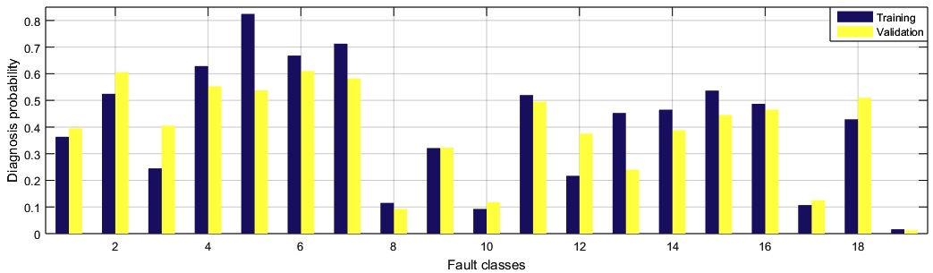
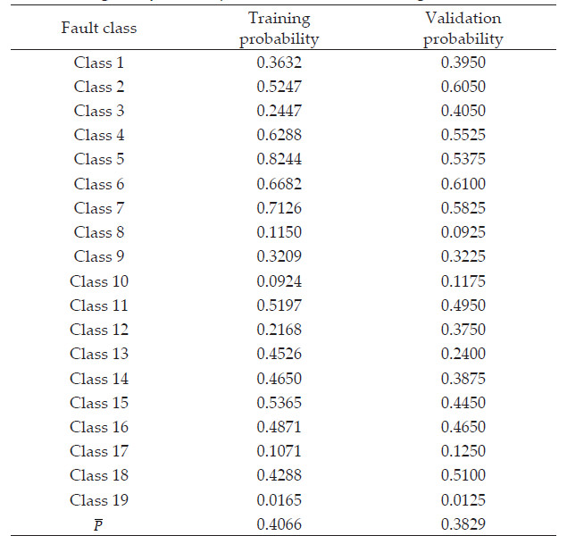
In order to have the highest diagnosis accuracy, two MLP parameters were tuned: the number of hidden layer neurons and the number of epochs. After performing different computations, 54 neurons and 2000 epochs produced the maximal validation probability. Figure 8 shows an example of this tuning. Figure 9 presents the diagnosis probability of each fault class for training and validation sets. Table 7 shows these values as well. For validation, the higher probabilities are obtained from classes 2, 6 and 7 (60.50 %, 61.00% and 58.25% of recognition respectively) while the lowest probabilities are produced by classes 8, 10 and 19 (9.25 %, 11.75 % and 1.25 % respectively). The differences between the probability values of both sets are explained by the limited pattern number of the validation set. The increase of this number can produce more accurate and closer results. The total diagnosis accuracy for training is 40.66% and 38.29% for validation.
Conclusions
The data generation using the software ProDiMES allowed the simulation of healthy and faulty conditions of an engine fleet in an appropriate environment facilitating the diagnostic process. This enabled the test of our diagnostic approach on the data of a new engine. The stage of baseline model testing permitted finding the best healthy engine performance approximation. This stage in an important part of the diagnosis process because it directly affects the diagnosis accuracy. After performing the calculations, the conclusion is that the baseline model selected has low level of errors and the deviations computed with this model adequately reflect engine health conditions. In the gas turbine fault recognition stage, the Multi-Layer Perceptron was used to classify the fault patterns. The results showed that this network correctly performs this task; however, the diagnosis accuracy for both sets (training and validation) seems to be relatively low. Some objective reasons of this could be: the great number of fault classes and the low fault severity randomly assigned to them. The other possible explanation is that we did not take into consideration all peculiarities of the engine simulation in ProDiMES because we are not authors of this simulator.
Future works can consider working with different recognition methods such as Radial Basis Network, Probabilistic Neural Network or Support Vector Machines in order to ensure that the fault recognition process was carried out correctly. The major issue is to increase the diagnosis accuracy.

