


 nova página do texto(beta)
 Inglês (pdf)
 Artigo em XML
 Referências do artigo
 Enviar este artigo por email
 Citado por SciELO
  Similares em
SciELO
Similares em
SciELO 
 Permalink
Introduction
A mixture experiment is one in which the response depends only on the relative proportions of the ingredients, or components, present in the mixture, this proportions represent the design variables. In such experiments, by mixing different components, the product is developed. Mixture experiments frequently appear in fields such as chemical, pharmaceutical, food and plastic industries. There are certain type of mixture experiments where the total amount of the mixture, or process variables, are involve too as a design variables (Piepel and Cornell, 1985; Goldfarb et al., 2004). In this paper, we focus on the mixture experiments with the proportions of the components as the only input variables.
If x i denotes the proportion of the ith of q components, then xi ≥ 0 for i = 1, 2,..., q, and
 (1)
(1)
Commonly the design region (1) is subject to additional constraints of the form
 (2)
(2)
to one or several components. These additional restrictions may result in extremely small range in terms of the mixtures. Not only does the experimental design region become constrained, but the resulting model from a mixture experiment also has to satisfy the constraint. This can cause difficulties in model fitting arising from ill-conditioning. That is, the columns of the corresponding model matrix can be almost linearly dependent (Prescott et al., 2002). Some consequences of ill-conditioning are that the least squares estimators of the parameters have large standard errors and are highly correlated, and the estimates are highly dependent on the precise location of the design points.
Data from a mixture experiment are usually modelled using Scheffe´'s polynomial models (Sheffé, 1958). The quadratic Scheffé's model has the general form:
Scheffe´'s model

where β i and β ij are unknown parameters to be estimated.
Because of the mixture constraint Eq. (1), the quadratic form of Scheffé's model involves linear terms and cross-product terms only, but this could be re-parameterized to include square terms (Philip and Norman, 2009). In fact, there are a number of different ways of writing a polynomial model, of any specified order, obtained by re-parameterization using the mixture constraint (Prescott et al., 2002).
Alternative polynomial model forms include the intercept models, which are obtained by replacing one mixture component, for example x q , for a constant term. A related model is the slack-variable model, in which one variable (designated the slack variable) is entirely eliminated by substitution; that is, by expressing it in terms of the remaining k - 1 components using Eq. (1), then substituting it into Scheffe´'s model (Piepel and Cornell, 1985). The different between the intercept model and the slack-variable model, is that the slack-variable model has quadratic model terms, while intercept model only present linear and interactions model terms, see (Cornell, 2000; Philip and Norman, 2009; André, 2005). Such re-parameterized models are equivalent in the sense that they lead to the same predicted values and basic analysis of variance (Philip and Norman, 2009). These two models are re-parameterizations of one another and all lead to the same fitted response contours and residuals. The equations may be expressed as follows, with the same symbols being used for parameters that are common to the different models:
Intercept mode
 (3)
(3)
Slack-variable model
 (4)
(4)
Moreover γ i = β i − β q , α i = β i − β q + β iq , α ii = −β iq and α ij = β ij − (β iq + β jq ).
The pros and cons of the use of intercept models or slack-variable models, as opposed to Scheffe´'s model, have generated a lot of discussions among research workers and practitioners (André, 2005). This issue was discussed by Cornell (2000), one of the questions raised by him was “does it matter which component is designated the slack variable?” He attempted to answer this question by discussing three numerical examples. In André (2005), the same issue was revisited from a different perspective. Emphasis was placed on model equivalence through the use of the column spaces of the matrices associated with the fitted models. It was shown that for the Scheffé's complete model and its corresponding slack-variable models, their reduced models, or submodels, provide different types of information. For some reduced models of a given size, Scheffé’s model may provide the best fit, but for other reduced models, some slack-variable models may be preferred. Prescott et al. (2002) propose an alternative pseudo-component-type transformation that leads to model coefficients that represent predictions at a wider selection of points within the design space. This delivers model coefficients that have a much more meaningful interpretation. Prescott and Draper (2002) compare the Scheffé model, the Kronecker model and the intercept model. Recently, Kang et al. (2015) propose a new criterion named “Correlation criterion”, to choose the best Slack-variable model using different components as slack variables, this criterion is only based on the design of the mixture.
In this paper, we analyzed if it matter which component is replaced for the constant term in the intercept model, in the sense on numerical stability. We also show by numerical examples that the Correlation Criterion, presented in Kang et al. (2015), does not work for the intercept model. Next, as suggested in the literature, we use linear transformation to alleviate the numerical instability. In addition, we try four transformation methods and choose the best one for the intercept model and the slack-variable model. Finally, we compare the intercept model with the slack-variable model based mainly on the prediction accuracy and numerical stability.
Method
Diagnostic measures
Below we briefly explain some diagnostic measures that help to detect or identify collinearity (Cornell, 2003; Montgomery and Voth, 1994; Prescott et al., 2002).
Multiple correlation coefficient
We define x
j
as the j
th
column of X and X
j
as the matrix that results when the column x
j
is deleted from X. Then
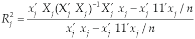 (5)
(5)
Where 1 is a column of unit elements.
When the column of constants of the X matrix is not available, the unadjusted multiple correlation coefficient can be obtained by
 (6)
(6)
For j = 1,..., p.
Variance inflation factor
The variance inflation factor (VIF) associated with the estimated regression coefficients β j is given by
 (7)
(7)
Small values of VIF are an indication of conditioning.
To evaluate the overall collinearity level of a model, it is propose the mean variance inflation factor (MVIF)
 (8)
(8)
where p is the number of effects in the model, excluding the intercept.
Condition number
Allow λ max > λ2 > ... > λ p−1 > λ min to be the p eigenvalue of X’ X, which are p solutions to the determinant equation

which is a polynomial with p roots.
There are many definitions of the condition number (CN) of a matrix. The general definition used in applied statistics is the square root of the ratio of the maximum to the minimum eigenvalues of X’ X denoted by
 (9)
(9)
Small values of λ min and large values of λ max indicate the presence of collinearity. Low values of the CN indicate some level of stability or conditioning in the least squares estimate.
Remedial measures
Linear transformation is suggested in the literature to alleviate the numerical instability. Below we briefly explain tree linear transformation.
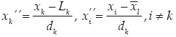
L-Pseudocomponents
When ingredients proportions x i are restricted by lower bounds L i while retaining an upper bound of 1, (Kurotori, 1966) recommended using L-pseudocomponents of the form
 (10)
(10)
Where L = ∑ L i . For the restricted mixture space to exist within the simplex, it is necessary that L < 1. Using the Eq. (10) in the pseudocomponent space, we have
 (11)
(11)
for i = 1,..., q (Prescott et al., 2002).
U-Pseudocomponents
When the range of each ingredient proportion x i is restricted by an upper bound U i only, Crosier (1984) recommended the use of U-pseudocomponents, defined as
 (12)
(12)
where U = ∑U i . For the U-simplex to be a region fully within the original simplex, it is necessary that U − 1 ≤ U min (Crosier, 1984). If is requirement holds, then the pseudocomponent transformation
 (13)
(13)
gives only positive multipliers of v i .
When U − 1 > U min , the U-simplex extend outside the original mixture simplex and better conditioning may or may not be achieved with U-pseudocomponents, depending on the particular restrictions and the design points.
Modified L-pseudocomponents
For the modified L-pseudocomponent we have to calculate the average over the N observations,
 (14)
(14)
where

Is a scale constant (Philip and Norman, 2009).
Correlation criterion
Kang et al. (2015) propose a new criterion named “Correlation criterion”, to choose the best Slack-variable model using different components as slack variables. Below we present de Correlation criterion.
Denote F as the design matrix for the mixture experiment of total q components and n experimental settings. Define r ij as the correlation between the ith and jth columns of F . This correlation is given by
 (15)
(15)
where F (,i) is the ith column of
F
,
 (16)
(16)
The matrix H is H = I − 1/n 11’and I is the n ⨯ n identity matrix. Thus, we choose the component that has the largest
Results and discussion
Four examples to evaluate de correlation criterion in the intercept model
In this section, we compute the correlation criterion in four examples chosen from the literature.
Example 1
We consider the example used by Cornell and Gorman (2009) involving three components and seven design points in the reduced region constrained by the inequalities

Foremost, we compute the correlation criterion. The calculations are presented below
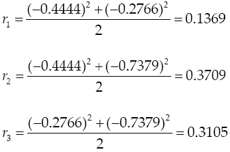
According to the correlation criterion x 2 should be replaced by a constant term. In Table 1 and Table 2 we present the VIF associated with the estimated regression coefficients, MVIF and CN for the three intercept models and the three slack-variable models respectively. We use the expression IM xi to represent the intercept model replacing x i for a constant term and SV xi to represent the slack-variable model using x i as a slack variable. It can be seen in Table 1 that replacing the component with the largest correlation by a constant term, the most stable intercept model is not achieved. On the other hand, it can be seen in Table 2 that choosing the component with the largest correlation criterion as slack variable, the most stable slack-variable model is achieved.


Example 2
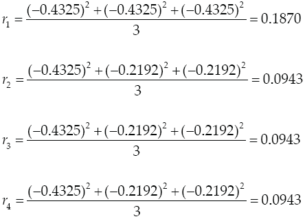
Cornell (2000) considered a three-component, mixture experiment example involving the tint strength of house paint blends. A simplex-centroid design was chosen with the simplex centroid replicated three times. In this example, if we proceed to compute the correlation criterion, we going to see that the value of r i is the same for the three components (see Tables 3 and 4). Thus, in this case the correlation criterion does not help to decide which component should be replaced for the constant term or should be selected as slack-variable.


Example 3
Cornell and Gorman (2003) present a numerical example with three component, ethanol (x 1), water (x 2) and propylene glycol (x 3). Experiment consist in seven-point design. Constraints on the component proportions were: 0.15 ≤ x 1 ≤ 0.50, 0.20 ≤ x 2 ≤ 0.70, 0.15 ≤ x 3 0.65. As can be seen in Table 5, again the correlation criterion dose not determine the most stable intercept model.


Example 4
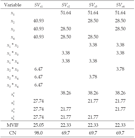
Cornell (2002) present an example named The Formulation of a Tropical Beverage. A tropical beverage was formulated by combining juices of watermelon (x 1), orange (x 2), pineapple (x 3), and grapefruit (x 4). In this example, the component with the largest r i is x 1, however, as can be seen in Tables 7 and 8, the most stable intercept model is achieved replacing component x 2, and the most stable slack-variable model is achieved using any of the three x 2, x 3 and x 4 components.
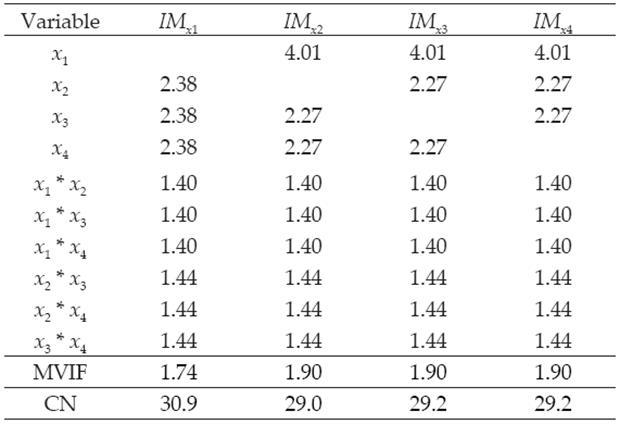
To summarize this section, we can point out that the intercept model can be used, in order to alleviate the collinearity problem. As could be seen in the examples shown in this section, the choice of which component is replaced for the constant term is crucial in the sense on numerical stability. However, the choice of which component should be replaced for a constant term, cannot be performed according with the correlation criterion. We recommend practitioners directly construct each possible intercept model matrix and choose the best one according to maxVIF, MVIF and CN criterion.
Linear transformations
To analyze mixture experiments, it is suggested to perform some linear transformation on the components’ proportions to reduce the ill-conditioning problem. However, different transformation methods work the best for different mixture models. For the slack-variable model, Kang et al. (2015) recommend scale the design of the proportion into [-1, 1], which is the typical scale used in classical design and analysis of experiments. For other mixture models L-, U- and modified-pseudocomponent transformations are recommended for the literature. Thus, we try all four transformation methods and choose the best one for the intercept model and the slack-variable model.
Example 5
In this example, we used the Example 1 data (Cornell and Gorman, 2009) and applied the four transformation, in order to choose the best one according to maxVIF, MVIF and CN. Based on Table 9, for this example, scaling the components’ proportions into [-1, 1] range works the best for the two models. In this case, the slack-variable model is the most parsimonious model.

Example 6
For the Example 6, we used the Example 4 data (Cornell, 2002) and applied the four transformation, in order to choose the best one according to maxVIF, MVIF and CN. Based on Table 10, for this example, the modified L- Pseudocomponent transformation works the best for the intercept model while scaling the components’ proportions into [-1, 1] range works the best for the slack-variable model. In this case, the intercept model is the most parsimonious model.

Numerical stability and prediction accuracy comparison
The choice of model forms can affect the numerical stability of the information matrix. In this section, we compare the intercept model with the slack-variable model based mainly on the prediction accuracy and numerical stability.
Example 7
In this section, we use the example presents in John (1984), the experiment involves an additive x 1 and three lubricant blends x 2, x 4 and x 4. The component proportions need to satisfy

First, we use different transformation methods for the two models and choose the best one according to maxVIF, MVIF and CN in Table 11. According to Table 11 scaling the components’ proportions into [-1, 1] range works the best for both models. In this case, the slack-variable model is the most parsimonious model.
Table 11 Comparison of the complete IM model and SV model using the Example 7 data, with different transformation.

In Table 12 we present the analysis of variance (ANOVA) for the slack-variable model using Example 7 date and scaling the components’ proportions into [-1, 1] range. As can be seen in Table 12, the interaction x
2, x
4 and the quadratic term

On the other hand, in Table 13 we present the ANOVA for the intercept model using Example 7 date and scaling the components’ proportions into [-1, 1] range. As can be seen in Table 13, the intercept terms x 2, x 4 and x 3, x 4 have no statistical significance effect over the response according with P-value at 99% confidence level. Thus, again we can removed both terms from the model.

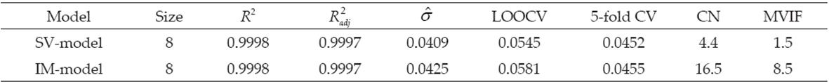
Table 14 shows the comparison of the reduced slack variable model and the intercept model.
R
2 and
Conclusion
In this paper, we analyzed if it matter which component is replaced for the constant term, in the intercept model, in the sense on numerical stability. By numerical examples, in section: Four examples to evaluate de correlation criterion in the intercept model we showed that the intercept model can be used to reduce the ill-conditioning problem. In addition, evidence was given that the choice of which component is replaced for the constant term is crucial in the sense on numerical stability. Moreover, we computed the correlation criterion and we determined that this criterion does not work for the intercept model, that is, the choose of which component should be replaced for a constant term, cannot be performed according with the correlation criterion. We recommend practitioners directly construct each possible intercept model matrix and choose the best one according to maxVIF, MVIF and CN criterion.
In section: linear transformations we tried four transformation methods and choose the best one for the intercept model and the slack-variable model. Scaling the components’ proportions into [-1, 1] range works the best for the slack-variable model, the modified L-Pseudocomponent transformation works the best for the intercept model in some cases.
Finally, in section: numerical stability and prediction accuracy comparison we compare the intercept model with the slack-variable model based mainly on the prediction accuracy and numerical stability. The slack-variable model has the best prediction accuracy and is the most parsimonious model in terms of numerical stability.

