


 nueva página del texto (beta)
 Inglés (pdf)
 Artículo en XML
 Referencias del artículo
 Enviar artículo por email
 Citado por SciELO
  Similares en
SciELO
Similares en
SciELO 
 Permalink
Introduction
The numerous geotechnical borings performed in the urban area of Mexico City can be used to obtain a better knowledge of the subsoil and for improving the accuracy of the existing geotechnical zoning map for regulatory purposes of construction (GDFa, 2004; GDFb, 2004).
To take advantage of the available information, computational and informatics tools, such as Geographical Information Systems as well as powerful mathematical tools based on Geostatistics have been used. Geographic Information Systems are useful to organize geotechnical information for fast and easy reviewing. On the other hand, Geostatistics, defined as the application of random functions theory to the description of the spatial distribution of properties of geological materials, provides valuable tools for estimating data such as thickness of a specific stratum, or local value of a given soil property, taking into account the correlation structure of the medium. Additionally, uncertainty associated to these estimations can be quantified.
In recent years, several studies dealing with the subsoil characterization for different areas within the Valley of Mexico have been published. In that studies, Geostatistical methods have been widely used to assess the spatial distribution of geotechnical properties (Jiménez, 2007; Valencia, 2007; Hernández, 2013; Eyssautier, 2014; Juárez, 2014). The results of these works have been taken into account in the geotechnical zoning proposed in this paper.
Location of study area
The study presented in this paper is focused on the area shown in Figure 1. It includes parts of political delegations Álvaro Obregón, Azcapotzalco, Benito Juárez, Cuauhtémoc, Gustavo A. Madero, Iztacalco, Miguel Hidalgo and Venustiano Carranza in the Distrito Federal and municipalities of Naucalpan, Ecatepec, Nezahualcoyotl, Tlalnepantla in the Estado de Mexico (Figure 1).

Basic information
To characterize the geological formations and soil deposits typical of Mexico Valley subsoil, it was considered necessary to collect data of very different nature and to integrate and present this information in synthetized form.
Topography
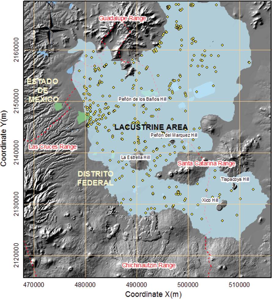
Figure 2 shows a Shaded Relief Model (SRM) illustrating the topographic configuration of the area. The model was built from the electronic data edited by Instituto Nacional de Estadística Geografía e Informática (INEGI, 2010).

Mexico Valley is a former lacustrine area limited by large topographic elevations: Sierra de Las Cruces, Monte Alto and Monte Bajo to the west reaching an altitude of up to 3600 m, Sierra de Guadalupe to the north reaching an elevation of 2960 m, the eastern Sierra Nevada and the Sierra de Chichinautzin to the south reaching an altitude of 3800 to 3900 m. Within the valley, some isolated volcanic domes such as Peñón de los Baños (2288 m), Peñón del Marqués (2372 m), Cerro de la Estrella (2443 m), Cerro de Xico (2348 m), Cerro de Tlapacoya (2442 m) and those forming Sierra de Santa Catarina (2482 m) protrude from the lacustrine area.
Geology
Figure 3 shows a geological map of the area (Mooser et al., 1966).

The central portion of the area consists of lacustrine soft clay deposits (Ql), which are surrounded by alluvial deposits (Qal) that also extend below the lacustrine deposits.
North of the area, the Sierra de Guadalupe range is formed mainly of andesitic and dacitic strato-volcanoes topped by acids domes that were formed in their final activity.
On the west side, the Sierra de las Cruces range is constituted by a line of large volcanoes oriented from NW to SE; the final activity of these volcanoes was of explosive type leading to the formation of extensive volcanic fans constituted by pyroclastic materials (T) associated with that activity.
On the east side, the Sierra de Santa Catarina range is formed by a line of volcanoes oriented in the WE direction; those are very young volcanoes, so that their eruptive products are lavas (Qv) that are interbedded with alluvial (Qal) and lacustrine (Ql) deposits.
Finally, in the south, the Sierra Chichinautzin range is an extensive volcanic field of the quaternary formed of many individual bodies, whose volcanic products, mainly lavas (Qv), form a huge mass of rock that separates the Mexico basin from the Cuernavaca valley.
Geographic information system for geotechnical borings
To assess the configuration of typical layers of the subsoil it was taken advantage of the profiles of geotechnical borings provided by public institutions and private contractors. These borings profiles have been incorporated into a Geographic Information System developed by the Geocomputing Laboratory of Institute of Engineering, UNAM (Auvinet et al., 1995).
The Geographic Information System for Geotechnical Borings (GIS-GB) for the study area has been built using ArcMap ver. 9.2 (commercial software). Nowadays, the system includes a database with information on more than 10000 borings (type, date, location, depth, water table level, etc.) and a database of images of geotechnical profiles, which can be readily consulted (Figure 4).

Incorporating information from the borings in the system requires pre-processing: the information is critically reviewed and converted from analog to digital format of either raster (cell information) or vector (digitized information) type.
Subsoil model
Vertical model
The typical soil profile sequence in the lacustrine zone of Mexico City subsoil includes a thin superficial Dry Crust (DC), a First Clay Layer (FCL) several tens of meters thick, a First Hard Layer (FHL), a Second Clay Layer (SCL) and the so-called Deep Deposits (DD) (Marsal and Mazari, 1959).
Horizontal model
Article 170, Chapter VIII, of Mexico City Building Code (GDFa, 2004), establishes that for regulatory purposes, Mexico City is divided into three zones with the following general characteristics:
Zone I. Hills, formed by rocks or hard soils that were generally deposited outside the lake area, but where sandy deposits in relatively loose state or soft clays can also be found. In this area, cavities in rocks, sand mines caves and tunnels as well as uncontrolled landfills are common.
Zone II. Transition, where deep firm deposits are found at a depth of 20 m or less, and consisting predominantly of sand and silt layers interbedded with lacustrine clay layers. The thickness of clay layers is variable between a few tens of centimeters and meters.
Zone III. Lake, composed of potent deposits of highly compressible clay strata separated by sand layers with varying content of silt or clay. These sandy layers are firm to hard their thickness varies from a few centimeters to several meters. The lacustrine deposits are often covered superficially by alluvial soils, dried materials and artificial fill materials, the thickness of this package can exceed 50 m.
Theoretical concepts of geostatistics
To define with better precision the boundary between zones II and III, a contour map for the thickness of soft clay deposits, also corresponding to the depth to the Deep Deposits was constructed, using geostatistical techniques. The basic concepts used for this type of analysis are presented in this section.
Random field (Auvinet, 2002)
It has been proposed to consider spatial distribution of soil properties and geometrical dimensions of soil strata as realizations of random fields (Matheron, 1965; Auvinet, 2002). This hypothesis makes it possible to use the mathematical tools of the random function theory for important applications such as estimation of the variables of interest in a specific point or volume where no measurement have been performed.
Consider a geotechnical variable V(X), either of physical (i.e. water content), mechanical (i.e. shear strength) or geometrical nature (i.e. depth or thickness of some stratum) defined at points X of a given domain R p (p = 1, 2, or 3). In each point of the domain, this variable can be considered as random due to the range of possible values that it can take (Figure 5). The set of these random variables constitutes a random field (Vanmarcke, 1983).

Structural analysis
To describe a stationary random field, the following parameters and functions are generally used (Matheron, 1965; Deutsch, 1992; Auvinet, 2002)
Expected value
 (1)
(1)
Variance
 (2)
(2)
Autocovariance function
 (3)
(3)
Where
h |
= distance between two points X and X + h u of the domain |
u |
= unit vector in the considered direction |
N |
= total number of data |
N(hu) |
= number of data pairs separated by a distance h in direction u within appropriate tolerance in tervals |
The autocovariance function, commonly anisotropic, represents the degree of linear dependence between the values of the property of interest in two different points. It can be written in the form of a coefficient of autocorrelation without dimension whose value is always between -1 and +1
Correlation coefficient
 (4)
(4)
The autocovariance and the correlation coefficient are not intrinsic properties of the two points X and X + h u, they also depend on the population, that is to say, on the domain in which the field is defined.
Correlation distance
The correlation distance (also known as Reach, Influence or range) is the distance beyond which variables V (X) y V (X + h u) are no longer correlated.
The correlation distance, δ(u)= 2a(u), is conventionally estimated from the experimental correlogram, as:
 (5)
(5)
where: h c is the first value of h for which ρ v (h u) is equal to zero.
Estimation
Geostatistics can be used to estimate the value of a property of interest at points of the medium where no measurement has been made. It is then possible to interpolate between available data and to define virtual borings, cross-sections or configurations of a given stratum within the soil. The problem can be generalized to the estimation of the average value of a property in any sub-domain of the studied medium, for example, in a given volume or along a certain potentially critical surface.
To reach this objective, linear statistical estimators without bias and with a minimum variance can be used (Best linear Unbiased Estimation or “BLUE”). This technique, also known as Ordinary kriging (Krige, 1962; Matheron, 1965; Vanmarcke, 1983 ; Deutsch, 1992; Auvinet, 2002) is also widely used in mining engineering. The estimate is
 (6)
(6)
The value of the (minimized) variance error associated to the estimate, also known as “estimation variance” can also be assessed
 (7)
(7)
Configuration of deep deposits depth
Definition of the random field
The geotechnical zoning map is based on the subsoil models previously described. In the context of the geostatistical analysis, the depth of Deep Deposits (DD) is considered as a random field V(X), distributed within an R P domain, with p = 2 (area of the former lacustrine zone as defined from topographical and geological information). The set of measured values within the R P domain (Figure 6) is considered as a random sample of this random field. A structural analysis aimed at defining the field parameters was performed after removing a linear trend to obtain experimental correlograms and correlation distances. Theoretical correlograms were fitted to the data set.
Statistical description
Accepting the ergodic hypothesis for the random field in study, the main statistical parameters of the depth of the deep deposits were estimated (Table 1). In Figure 7 the variability of the data is described graphically by means of a histogram.


Structural analysis
Trend analysis
The general trend of the Deep Deposits depth was assessed by means of a linear regression analysis, fitting an equation of the form:
V(X) = ax + by + c to the data. The coefficients that best describe this trend are:
a = -0.00096398, b = 0.00064913 and c = -955.997663.
The corresponding linear regression surface (Figure 8) helps to identify the preferential direction of variation of the random field. The figure shows that the values of the Deep Deposits depth decrease from northwest toward the southeast. The presence of this trend is taken into account to calculate the experimental correlograms and in the estimations.

Estimation of the autocorrelation coefficient function
After removing the trend from the original data, a residual field was obtained. The autocorrelation coefficient function was calculated along four preferential directions with azimuth Az = 0°, 45°, 90° and 135°, and steps (Δh) of 250m (Figure 8). These functions describing the correlation structure are shown in Figure 9. The correlation distances (δ) obtained for each preferential direction are shown in Table 2.


It can be seen that influence distances are of the order of several thousand meters. Some anisotropy is detected. Figure 9 shows that the shortest correlation distance of 4500m corresponds to directions Az = 0° and 135° and the highest correlation distance of 600m to direction Az = 90°.
The experimental correlograms were fitted to an exponential function to obtain the spatial correlation model.
 (8)
(8)
Estimation
The expected value and estimation standard deviation of the depth of the Deep Deposits were obtained at all nodes of a regular grid conveniently defined, using the technique of Ordinary Kriging (Deutsch and Journel, 1992).
Conservatively, a correlation distance δ = 5000m was considered in direction Az = 45° and δ = 4500m in direction Az = 135°. The final estimate of the field was obtained reinstating the linear trend into the results. Additionally, the estimation variance was obtained.
Visualization
From the results, a contour map was built showing the spatial distribution of the depth of this layer within the studied area (Figure 10). The results of the estimation can also be represented by a surface map, assigning the value of the depth to the vertical coordinate (elevation) of each point (Figure 11).


Figures 10 and 11 show that the largest Deep Deposits depths are located in the area of the former Chalco Lake, in the south part of the lacustrine area. In this area, the Deep Deposits depth reaches values as high as 90 and 100m.
Geotechnical zoning map
The map of Figure 10 has immediate practical implications, and is useful to update the geotechnical zoning map of Federal District. The curves of equal depth of Deep Deposits are also useful in earthquake engineering to evaluate the site effects expected at some specific place.
Taking into account the definition of the transition zone previously indicated (GDFa, 2004) and using the map of Figure 10, it was possible to define the boundary lines between zones II and III. After defining this boundary line and making the appropriate settings, the new geotechnical zoning map, shown in Figure 12, was build. This map has been proposed for integration into the Building Code.
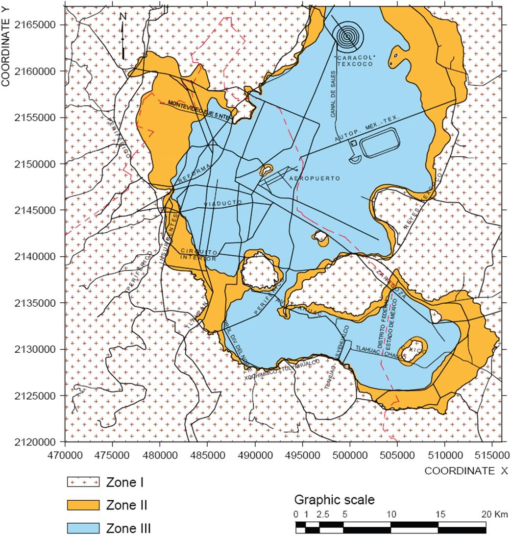
The purpose of this map is to contribute to improving the current geotechnical zoning map and establishing more precise boundaries to help better define the location of different soil types in the Valley of Mexico. However, it is necessary to remark that the map should be updated in periodic form, integrating the new available information.
It should also be stressed that the geotechnical zoning map only provides a general orientation and in no case should be used to avoid the traditional geotechnical surveys of geotechnical that must be performed for each project as required by the building code.
Conclusions
Recent advances in the geotechnical characterization of the subsoil of Mexico Valley using a Geographic Information System for Geotechnical Borings (GIS-GB) that includes more than 10,000 soil profiles have been presented.
Geostatistical techniques were used to define a model of the compressible lacustrine soils lower boundary also known as Deep Deposits. It can be concluded that Geostatistical methods provide a rational tool for interpreting the available geotechnical information and to evaluate the spatial variability of the subsoil. They can be useful to eliminate a large part of the subjectivity generally introduced in traditional stratigraphical interpretations and will certainly be used much more frequently in the future.
The availability of increasingly accurate information about the distribution of materials and index and mechanical properties in Mexico Valley subsoil has immediate implications for updating the building code and for planning of future works and is deemed to be useful for civil engineers working in the area.
The geotechnical zoning map shown in this paper only provides a general orientation and in no case should it be used to avoid the traditional geotechnical surveys studies that must be performed for each project as emphasized in the building code.

