


 text new page (beta)
 English (pdf)
 Article in xml format
 Article references
 Send this article by e-mail
 Cited by SciELO
  Similars in
SciELO
Similars in
SciELO 
 Permalink
Introduction
Recent developments of high performance electronic equipment have led to a general reduction of spacing and increase in power. This fact has created a need for efficient heat dissipation. In response to this demand, miniature-size compact heat exchangers with capacity to operate as efficient heat sinks have been recently developed. The reduction of channel size is now a reality and mini-tubes with hydraulic diameters from 200 μm to 3 mm are commonly used. The problem, however, is that the heat transfer and pressure drop in this kind of systems may be significantly different from what has been reported in conventional size evaporators, and there is a lack of reliable information about the thermal performance of these devices.
Much of the progress of heat transfer has been driven by the necessity to predict the performance of a thermal system, which results from applications of fundamental laws (mass, momentum, and energy conservation) for basic problems, supplemented with empirical correlations for more complex cases (complexities stemming from system geometry, flow conditions and appearance of simultaneous heat transfer mechanisms). Unfortunately, there are critical applications related to energy efficiency, environmental impact, optimal system design and control, where traditional techniques fail to provide an adequate prediction and more advanced prediction methods are required. While the thermal sciences must continue to gradually increase knowledge and insight of fundamental phenomena, there are some new technologies, such as artificial neural networks (ANNs) that can be used as application tools to supplement such understanding. This is particularly true in the case of complex flow situations occurring in novel applications, such as the cooling of electronic devices with miniature size evaporators.
Heat transfer prediction of condensation and evaporation processes in refrigeration and air conditioning units is a complex task when compared to the prediction of single phase heat transfer. Traditional powerlaw correlations have proved to be inaccurate for this kind of processes, even though there is a need of good predictions in these applications. For instance, using their correlation for forced convective boiling, Gungor and Winterton (1986) obtained errors of 21.4% for saturated boiling and 25% for sub-cooled boiling with respect to their own measurements. Years later, it was shown that when experimental data from other authors are used, the errors from this and other correlations can be as large as 50%.The process of phase change in pipes undergoes a series of flow regimes, which go from single phase flow, onset of bubble formation, annular flow boiling, film boiling, mist flow and superheated vapor flow, depending on mass flow rate, degree of superheating, pressure, tube diameter, orientation and vapor quality. All these phenomena occur over a short pipe length. The inability of power-law correlations to catch up with all these phenomena occurring during two phase convection lies as the reason for the inaccuracy of the predictions.
One of the modern technologies that have been successful as an analysis tool is the technique of artificial neural networks (ANNs). This technique has been applied for pattern recognition, decision making, control systems, information processing, symbolic mathematics, computer vision and robotics. The use of ANNs has been extended to a wide variety of disciplines, among which are the thermal sciences, because it allows the study of complex thermal systems that otherwise would be impossible to characterize with conventional analysis techniques, since they offer an alternative approach for experimental data compression. ANNs have been used for the prediction of heat transfer coefficients (Jambunathan et al., 1996), the calculation of Nusselt numbers (Thibault and Grandjean, 1991), the prediction of heat transfer in heat exchangers (Díaz et al., 1999; Pacheco-Vega et al., 2001a, 2001b), the estimation of heat transfer in the transition region of a circular tube (Ghajar et al., 2004), to study the thermal performance of cooling towers (Islamoglu, 2005), to analyze phase change in finned tubes (Ermis et al., 2007), to compute friction and heat transfer in helically-finned tubes (Zdaniuk et al., 2007), to model evaporative air coolers (Hosoz et al., 2008), finned-tube condensers (Zhao and Zhang, 2010), finned-tube evaporators (Zhao et al., 2010), and indirect evaporative cooling (Kiran and Rajput, 2011). One of the main advantages of ANNs is that they do not require a detailed knowledge of the physical phenomena describing the system under analysis.
The objective of this work is to use ANNs to characterize the convective heat transfer rate occurring during the evaporation of a refrigerant flowing inside tubes of very small diameter. For this purpose, an experimental setup of a mini-tube evaporator with a constant heat flux condition is first built and instrumented. Next, the experimental apparatus is used to acquire the measurements necessary to map the thermal performance of the evaporative process inside a bundle of mini-tubes as functions of flow and thermal operating conditions and geometrical parameters. Finally, using the experimental data, several neural network configurations are trained and the most accurate was selected to predict the thermal behavior of the mini-tube evaporator. The results reveal that ANNs are accurate predictive tool for the analysis of complex systems such as mini-tube evaporators.
Artificial neural networks
The theory under which ANNs work is based on the structure and functionality of biological neural systems, where the neuron is the fundamental element. The biological neuron, schematically shown in Figure 1, is formed by the body of the cell, an axon and a series of dendrites. The axon transports the incoming signal from a neuron to other neurons, whereas the dendrites provide enough surface area to facilitate connectivity with other neurons. ANNs have nodes (or artificial neurons), as shown in Figure 2, whose function is to make mapping operations between inputs and outputs. This mapping is usually done by means of a sigmoidal function, although other functions (e.g.: hyperbolic tangent or Gaussian) have also been successfully applied. These artificial neurons are connected to others through linkages of the type axon-synapsis-dendrite, each associated with a weight. As in the case of a biological synapsis, this weight determines the nature and intensity of the influence of a node on another. A weight of large value (either positive or negative) corresponds to a large excitation, while a small weight corresponds to a negligible one. There exist different neural network configurations, the fully-connected being the most common in the analysis of engineering problems. This type of ANN, also called multilayered perceptron or feed-forward network, is shown schematically in Figure 3. It has a series of layers, each formed by a set of nodes; the first layer is called input layer; the last one is the output layer, and the inner layers are known as hidden layers. The network configuration shown in the figure is referred to as fully-connected since each node of a layer is connected to all the nodes of adjacent layers.


To build an artificial neural network model, a training process must be carried out first. This process is accomplished by adjusting the synaptic weights and biases when the different values of input and output variables are supplied to the network. The technique for training the ANN is that of back propagation, described by Rumelhart et al. (1986). After the network configuration has been chosen, the first step of the algorithm is to randomly assign initial synaptic weights and biases. The second step, known as feed-forward step, starts by feeding the data onto the first layer (input layer). The information resulting from the input-output sigmoidal mapping at each node of the inner layers is then transferred forward until it reaches the nodes of the last layer (output layer), where the outputs from the network are compared with the experimental data, and their differences are used later to adjust the corresponding weights. This step is known as back-propagation. In it, the error generated from the feed-forward phase is quantified in each layer and each node by means of a delta rule and propagated backwards to change the synaptic weights and biases. A feed-forward step followed by a back-propagation one comprises a cycle. The training process ends when the error in the last cycle decreases below an established threshold value.
Experimental setup and procedure
Experimental set up
An experimental apparatus based on the inverse Rankine cycle, which includes a test section for evaporation of a refrigerant inside a set of mini-tubes, was built and instrumented. The test bench is shown schematically in Figure 4. It has two fluid circuits: one for the refrigerant R-134a and one for cooling water. The refrigerant circuit incorporates a refrigerant pump (RP), a pre evaporator (PE), an evaporator test section (TS), an expansion valve (EV), a double pipe condenser (DC) and sub-cooler (SC) -in which the refrigerant flows inside the annular section while chilled water flows inside the circular pipean accumulator tank (AT), a flow meter (FM), a dryer filter (DF) and several peepholes (PH). This circuit starts in the container (CO) and refrigerant flows toward the pump. This is a 1/13 HP rotary positive-displacement type pump with external gears, magnetic coupling, and provides volumetric flow rates from 4 to 458 l/h. The pump circulates the refrigerant through a Coriolis-type flow meter, which measures mass flow rates from 0 to 65 kg/h, densities from 0.1 to 2.9 g/cm3, and temperatures from -50°C to 180°C. After the flow meter the refrigerant flows to a pre-evaporator, leaving it at the specific vapor quality required at the entrance of the evaporator test section.

This experimental setup has an electrical resistance through which the power is supplied to the system that is controlled by means of a variable autotransformer. Both the pre-evaporator and the test section have similar designs (see description below). Once the refrigerant is pre-heated, it is circulated through the evaporator test section, where it evaporates and the required measurements for the present study are collected. After passing an expansion valve, a condenser and a subcooler are used to treat the refrigerant that leaves the test section before it returns to the accumulator tank. The condenser and the sub-cooler are concentric-tube heat exchangers, shown schematically in Figure 5, in whose annular sections chilled water is circulated. The chiller (CH) has a temperature range from -10 to 40°C, and a volumetric flow rate up to 4.2 l/min. A bypass circuit is also included in order to adjust the average flow rate. The pressure in the test section is measured by means of a pressure transducer, which has a range from 0 to 1 MPa. The pressure is regulated varying the temperature and flow rate of water in the condenser. The input and output temperatures are measured with J-type insulated thermocouples.

Pre-evaporator and evaporator test section design
Figure 6 shows the test section formed by a collinear array of 20 adjacent copper tubes, each having a 3.175 mm outer diameter, 1.75 mm inner diameter and 1.5 m length. The array of tubes is sandwiched between two 90 cm long, 7 cm wide and 4.8 mm thick copper plates. Six J-type thermocouples were inserted along the collinear array in the gaps formed between tubes and the copper plates. In order to reduce the contact thermal resistance, the space between the copper tubes and the plates was filled with conducting silicon paste. Each copper plate is covered with a stainless steel lamina that has 11 cuts, as shown schematically in Figure 7, to form a path for the circulation of an electric current that will generate heat by Joule effect (and will apply it to the system), which is regulated by adjusting the voltage applied with a 0-120 V CA variable autotransformer. A thin gypsum layer is placed as a plank between the copper and stainless steel plates to avoid electric currents through the copper plates and tubes. In order to reduce heat losses to the exterior, the outer side of the stainless steel plates is covered with two layers of asbestos tissue and a fiberglass layer.


The information obtained from the experimental runs was collected with a data acquisition system that includes a National Instruments SC-2345 portable modular system, a data acquisition card NI DAQCard6036E for PCMIA, thermocouple modules NI SCC-TC, and a current module NSC-C120. The program Measurement and Automation Explorer is used to obtain data and process them in a PC.
Data collection and processing
The refrigerant mass flow rate, the system pressure, the applied heat flux generated from the electrical resistance and the incoming refrigerant vapor quality entering the test section were varied during the experiments. The refrigerant mass flow rate was varied by adjusting the operating conditions of the refrigerant pump and the bypass. The system pressure was varied by injection of refrigerant into the system. As indicated above, the magnitude of heat flux applied was varied by adjusting the variable autotransformer position. The vapor quality of the refrigerant entering the test section was controlled by the amount of heat provided in the preevaporator.
The following parameters were measured during the experimental runs:
Ts = test section tube surface temperature
Tf = average refrigerant temperature during evaporation
Tpre = pre-evaporator refrigerant input temperature
P = system pressure
ṁ = refrigerant mass flow rate
V = applied voltage
I = applied current
The temperatures Tf and Ts are obtained from direct measurements with J-type thermocouples. With these measurements it is possible to calculate the experimental inner flow side convective heat transfer coefficient, U, as
where q" is the applied heat flux (applied electric power per unit surface area), which is a function of the voltage and current applied and controlled by the variable autotransformer, Ap is the copper plates surface area, and At is the external surface area of the tubes.
The vapor quality at the entrance of the test section was selected to be 20%; this was achieved by regulating the heat provided to the pre-evaporator, which is controlled by the variable autotransformer position. The vapor quality at the exit of the test section was selected to be 80%; this was also achieved by regulating the heat provided to the evaporator.
The amount of heat needed to achieve a vapor quality of 20% as entrance condition to the evaporator, expressed as the product of voltage by current circulated through the pre evaporator, is determined by
where h2 is the enthalpy of refrigerant that is 20% vapor at the pressure of the test section, and can be determined by h2=hf+x2hfg ; hf is the saturated liquid enthalpy of the refrigerant at the evaporator pressure, hfg is the latent heat of evaporation of the refrigerant at the evaporator pressure and x2 is the quality, in this case x2 = 0.2.
The amount of heat needed to achieve a vapor quality of 80% as exit condition of the evaporator, expressed as the product of voltage by current circulated through the evaporator, is determined by
where h3 is the enthalpy of refrigerant that is 80% vapor at the pressure of the test section, and can be determined by h3 = hf + x3hfg ; hf is the saturated liquid enthalpy of the refrigerant at the evaporator pressure, hfg is the latent heat of evaporation of the refrigerant at the evaporator pressure and x3, is the quality, in this case x3 = 0.8.
Results and discussion
Three parameters were chosen as relevant input data for the characterization of the
refrigerant evaporation in the mini-pipe heat exchanger described before. These are:
saturation temperature during the evaporation process (Tsat
), refrigerant mass flow rate (ṁ), and applied heat flux
(q''). The output obtained from this information is the
experimental convective heat transfer coefficient
A number of 177 measurements of Tsat
, ṁ and q'' were obtained to calculate
where

The number of cycles during training was defined in terms of the minimum value of the maximum error and standard deviation. An example of the behavior observed for this error is shown in Figure 8 for the case of the neural network 3-13-1. From the observations of this and other cases not shown in the paper, where the same behavior occurs in all other configurations, it was concluded that after 10,000 cycles the reduction of the maximum error was negligible, and this number of training cycles was taken as the standard throughout this investigation. Importantly, depending on the problem at hand the training process may be computationally expensive but, as pointed out by Pacheco-Vega et al. (2001b), once the ANN has been trained, its subsequent use for predictions is immediate. For the problem at hand, in all cases analyzed the training process took less than 5 minutes of CPU-time per ANN model, which is an excellent processing time as compared to that necessary for the optimization process to find the typical correlation constants. From the table it can be seen that although the results for the 18 configurations are close, the 3-11-1 was the best in terms of the maximum error, while the 3-6-4-1 proved to be the best in terms of σ. Both configurations are close to the "best" configuration according to the ad-hoc criterion of Hecht (1987), which indicates that the configuration 3-7-1, shown schematically in Figure 9, should be the best. When searching for a more robust model, as mentioned before, there are other configurations that are very competitive. Configuration 3-5-3-1, with R=1.0000, σ=2.90E-4 and maximum error of 3.80, or configuration 3-3-1-1-1, with R=1.0000, σ=6.60E-4 and maximum error of 3.75, are very good options.
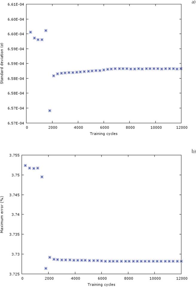
Figure 8 Evolution of a) standard deviation and b) maximum error as a function of the training cycle for the neural network configuration 3-13-1
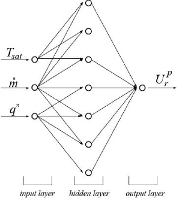
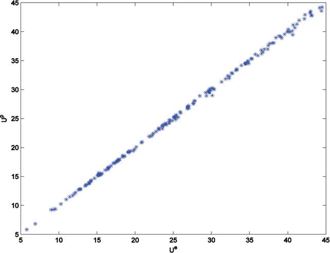
Figure 10 shows the convective heat transfer coefficient obtained experimentally,
Conclusions
The study of the physics involved in convective evaporation has increased its complexity since the appearance of enhanced surfaces for evaporators and new environmentally-friendly refrigerants. This enhanced complexity has made it more difficult to develop accurate correlations for the prediction of the thermal performance of evaporators. Reports in the literature clearly show that predictions based on models that consider forced convection and flooded evaporation as separate phenomena are severely degraded and new alternatives like artificial neural networks (ANNs) are necessary.
We have developed neural network models of a mini-tube evaporator that may be able to accurately predict the thermal performance under several operating conditions. Results obtained using the ANN technique, as developed in this investigation, are very promising. The prediction of heat transfer obtained in this work has a maximum error of 2.46% and a mean quadratic error of 0.51%, which is by far lower than the 30% obtained by other authors (Liu and Winterton, 1991), that use conventional correlation techniques. The technique of artificial neural networks is therefore an excellent option for reliable and precise characterization of thermal systems where evaporation processes occur, such as in refrigeration and air conditioning units, and when appropriately trained, the predictions obtained from neural network models are of the order of the experimental uncertainty.

