Selecting the Slack Variable in Mixture Experiment

 

Selección de la variable de holgura en experimentos para mezclas

 

Cruz-Salgado Javier

 

Universidad Politécnica del Bicentenario (UPB). Silao, Guanajuato. Correo: jcruzs@upbicentenario.edu.mx

 

Received: March 2015.
Accepted: April 2015.

 

Abstract

A mixture experiment is one where the response depends only on the relative proportions of the ingredients present in the mixture. There are different regression models used to analyze mixture experiments, such as Scheffé model, slack-variable model, and Kronecker model. Interestingly, slack-variable model is the most popular one among practitioners, especially formulators. In this paper, I want to emphasize the appealing properties of slack-variable model. I discuss: how to choose the component to be slack variable, numerical stability for slack-variable model and what transformation could be used to reduce the collinearity. Practical examples are illustrated to support the conclusions.

Keywords: condition number, mixture experiments, slack-variable model, scheffé model, variable transformation, Variance Inflation Factor (VIF).

 

Resumen

Un experimento para mezclas es aquel en donde la respuesta depende solo de las proporciones relativas de los ingredientes presentes en una mezcla. Existen diferentes modelos de regresión empleados para analizar experimentos para mezclas, tales como el modelo Shceffé, variable de holgura y Kronecker. Es interesante mencionar que el modelo de variable de holgura es el que goza de mayor popularidad entre profesionistas, especialmente formuladores. En este artículo, se enfatizan las atractivas propiedades del modelo de variable de holgura. También se discute cómo seleccionar el componente que deberá ser la variable de holgura, estabilidad numérica para el modelo de variable de holgura y qué transformación puede utilizarse a modo de reducir colinealidad. Ejemplos prácticos se ilustran para sustentar las conclusiones.

Descriptores: número condicional, experimentos para mezclas, variable de holgura, modelo Scheffé, transformación de variables, factor de inflación de la varianza (VIF).

 

Introduction

The development of products generated by the mixing of different components is a special case of the response surface methodology (Ralph, 1984 ). The experimenter may be interested in modeling a response variable as a function, where different predictor variables (components) modify the behavior of the response. Mixture experiments are performed in many product-development activities. Mixtures problem examples include assessing the octane index in gasoline blend components; measuring the compressive strength of a standard concrete block; blends of bread flours, consisting of wheat and various permitted additives; fertilizer, consisting of blends of chemical; wines, blended from several varieties of grapes, or several sources of similar grapes; and the measurement of the characteristics of a fish cake flavor made of a mixture of three types of fish.

Data from experiments using mixtures are usually modeled using quadratic Scheffe model (S-model) introduced by Scheffe (1958).

An alternative model, the quadratic Kronecker model (K-model), was introduced by Draper and Pukelsheim (1998). This model contains second order terms only and takes the form

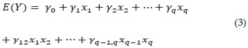
Another alternative model is the so-called Slack-Variable models (SV-model) which are obtained by designating one mixture component as a slack variable. The purpose of this model is to produce mixture models that depend on k-1 independent variables. The quadratic SV-model takes the form

These three models are re-parameterizations of one another and all lead to the same fitted response contours and residuals. There are a number of different ways of writing a polynomial model, of any specified order, obtained by re-parameterization using the mixture constraint, see Prescott et al.(2002) for a discussion of model specification and ill-conditioning. All such re-parameterized models are equivalent in the sense that they lead to the same predicted values and basic analysis of variance. However, the coefficients of the various terms in the models can be confusingly different and thus difficult to interpret Prescott et al.(2009).

In mixtures problems, the response variable depends only on the relative proportions of the ingredients or components of the mixture. Other types of mixture experiments involving the total amount of the mixture or certain process variables (Piepel and Cornell, 1985; Goldfarb et al., 2004; Kowalski et al., 2002) are out of the scope of this paper. These proportions are connected by a linear restriction

Commonly the design region (1) is subject to additional constraints of the form

to one or several components, these additional restrictions may result in extremely small range in terms of the mixtures. Further, mixture experiments with large number of ingredients may result in extremely small range too.

A general mixture model, in matrix terms, can be presented as Y = Xβ + ∈ or E (Y) = Xβ. To estimate the parameters in the β matrix via least squares the following expression can be used

Where the covariance matrix is V() = (X' X)^-1 σ² . The vector of fitted values is given by ŷ = Xβ and the residual vector is e = y - ŷ = y - X . Usually, the vector ∈ is assumed to follow a normal distribution, that is ∈ ∼ N (0, σ²).

If an exact linear dependence between the columns of X exist, that is, if there is a set of all non-zero c'_js such that

then the matrix X has a rank inferior to p (predictor variables), and the inverse of X' X does not exist. In this case many software packages would give an error message and would not calculate the inverse. However, if the linear dependence is only approximate, it is

then we have the condition usually identified as collinearity or Ill-conditioning (some authors use the term multicollinearity). In this case many software packages proceed to calculate (X' X)^-1 without any signal foreseeing to the potential problem.

When there is presence of Ill-conditioning computer routines used to calculate (X' X)^-1 can give erroneous results. In this case the least squares solution (6) may be incorrect. Moreover, even if (X' X)^-1 is correct, the variance of _s's, given by the diagonal terms in V() = (X' X)^-1 σ² can be inflated by Ill-conditioning (Ralph, 1984).

In this paper we investigated an alternative model for which functional forms are more appropriate than the S-model.

Prescott et al.(2002) show that the quadratic K-model is the quadratic model specification that is less susceptible to ill-conditioning than the S-model. They investigated which model form is best conditioned among all the possible variations of a second-order model obtainable by using different substitutions of the model restriction (4) into a full quadratic regression model. They also give their main theoretical results motivating their preference for the quadratic K-model. They concluded that the quadratic K-model always reduces the maximum eigenvalue of the information matrix compared with that of the S-model, but, the minimum eigenvalue does not necessarily increase.

Many practitioners and researchers alike profess to have been successful using the SV-model approach. When the presence of collinearity among the terms in S-models is a possibility and the appearance of the complete model form is of concern, the choice of using the SV-model makes sense. Reference to the SV-model form of the mixture model appears in Snee, (1973), Snee and Rayner (1982), Piepel and Cornell (1994) . Examples of the use of a slack variable found in the literature are Cain and Price (1986); Fonner et al. (1970) and Soo et al. (1978).

The pros and cons of the use of SV-models, as opposed to S-model, have generated a lot of discussions among research workers and practitioners. Snee and Rayner (1982) very briefly discussed using SV models as a way to reduce collinearity and test hypotheses of interest for mixture experiment problems. However, they concluded that the intercept forms of mixture experiment models (which they discuss) were preferable for hypothesis testing purposes. Piepel and Cornell (1994) discussed and illustrated several approaches for mixture experiments, including the SV approach. They used the four components shrimp patty data set of Soo et al.(1978) to compare the SV and mixture experiment approaches, and show how the SV approach yielded could misleading conclusions regarding the effects of the non-SV components. This issue was recently discussed by Cornell (2000) . One of the questions raised by him was "does it matter which component is designated the slack variable?" He attempted to answer this question by discussing three numerical examples. Both complete and reduced models were fitted to the mixture data. He noted that there are situations where fitting the SV-model is reported to be more satisfying to the user than fitting the S-model. Khuri (2005) discussed and examined the same issue discussed by Cornell (2000) from a different perspective. Emphasis is placed on model equivalence through the use of the column spaces of the matrices associated with the fitted models. It is shown that while complete S-model and its corresponding SV-models are equivalent, their reduced models, or submodels, provide different types of information depending on the vector space spanned by the columns of the matrix of the fitted model. For some reduced models of a given size, S-model may provide the best fit, but for other reduced models some SV- models may be preferred. Landmesser and Piepel (2007) analyzed data from several examples using the mixture experiment and SV approaches.

The motivation of this paper comes from the fact that there are no clear guidelines to help practitioners to decide which model is most suitable for use under certain circumstances. Especially in those cases where the SV-model appears to be the best alternative.

Although the SV-model is very popular among practitioners due its simplicity, is not so advocated by literature. Cornell (2000) argues that the idea behind using a SV-model undermines the fundamental property of mixture experiments, which is, that the relative proportions of the mixture components are not independent. Piepel and Landmesser (2009) mentions that practitioners who use the SV approach with traditional statistical methods, can be misled in making conclusions about the effects of mixture components and in developing models for response variables. Considering the relationships between SV and S-model would avoid misleading results and conclusions, but typically practitioners who use the SV approach do not consider these relationships.

The main objective of this paper is to promote the SV-model for mixture experiments showing its nice features and more importantly, we provide guidelines on how determine the slack variable.

The remainder of this paper is organized as follows. Section 2 presents the definition of the SV-model, its features and benefits, and the introduction of the concept of "filler" ingredient. In section 3 we propose a new criterion to determine which ingredient in the mixture has to be selected as a slack variable based on the correlation between the columns of the information matrix. In section 4 we introduce two alternative transformations for the SV-model, which make the SV-model a better conditioned model. Finally in section 5 the main conclusions are given.

 

Slack-Variable Model

Definition of the SV-model

In a mixture experiment with components x_i, (i = 1, 2, ... q) , the SV approach involves designating one of the components as the "Slack Variable", and designing the experiment and/or analyzing the data in terms of the remaining q -1 components. In this paper x_q is designated as the SV. Thus, x₁ to x_q-1 would be used to design the experiment, develop models for the response variable, and perform other data analysis.

The quadratic models in equations (1) and (2) are equivalent. This means the coefficients (and their estimates) in equation (2) is a simple function of the coefficient (and their estimates) Y₀, Y_i and Y_ii in equation (1), and vice versa (Cornell, 2000). In fact, for equation (2) and (1)

See Cornell (2002, Section 6.13) for more discussion of these relationships.

Hereafter when referring to any slack-variable model with component x_q being the slack component, we shall abbreviate the model using SV_xq.

In the SV approach, traditional experimental designs such as factorial, fractional factorial, central composite, Box-Behnken, and others are typically used (Myers et al., 2009).

 

Introduce the concept of "filler" ingredient

The SV approach is widely used by practitioners in many disciplines; however, there is limited information in the mixture experiment literature.

Snee (1973) discusses using the SV approach when one component makes up a large percentage (> 90%) of the mixture. He explains that "when a mixture experiment is designed and analyzed in terms of q-1 components, the scientist is interested in the effect of changes of the levels of the components with respect to the slack component.

Snee and Marquardt (1974) prefer the mixture experiment approach unless one component makes up "an overwhelming proportion" of the mixture. In that case, they say "it may not be appropriate to view the problem as a mixture problem." This advice might be appropriate if the SV has no effect and only the trace components have substantive effects.

The SV approach has been mentioned in the literature and by practitioners as being useful in four situations (Piepel and Landmesser, 2009 ). Situation 1 occurs when the SV component makes up the majority of the mixture (Snee, 1973). Situation 2 occurs when the SV plays the role of a diluent and blends additively with the remaining components in the mixture. The SV approach can yield misleading conclusions in this situation (Cornell, 2002; Section 6.5). Situation 3 occurs when there is not a natural SV, but the data analyst is willing to consider models using each of the mixture components as the SV (Cornell, 2000 and Khuri, 2005). Situation 4 occurs when the component selected as the SV has no effect on the response. An example of such a situation is when the SV component is an inactive "filler" and the other components are the active ingredients. In this situation, a mixture experiment approach can be used to verify the filler component has no effect on the response. Then, mixture compositions and mixture experiment models can be expressed using the relative proportions of the remaining components.

 

The advantages of the SV model

Some advantages of the SV-model are mentioned below:

• If a "filler" is involved, classic factorial experimental design methods can be applied to the other ingredients, if only lower and upper bounds and no other constraints are imposed on them.

• If at the design stage, the "filler" ingredient is identified. Proper designs can be used such that the quadratic SV model has the diagonal information matrix, thus has the best conditional number.

• If "filler" cannot be identified, choosing the suitable ingredient as slack variable, with a proper linear transformation, the information matrix of SV model has the smallest condition number (see Section 3).

• Slack variable has much clearer interpretation than the other mixture model. For example, the linear effect of an ingredient is the change in the response when this ingredient is increased for a certain amount while only the filler is decreased for the same amount, or the other way around.

• SV model is more suitable to perform variable selection, thus can lead to more accurate prediction on new data set. Scheffé model can have variable selection on the condition that all the linear effects are kept in the model. K-model is not able do variable selection.

• Much easier to use and understand, thus already very popular among formulators.

 

Choice of slack variable

As mentioned above, the information matrix of the mixture models can easily become ill conditioned. Collinearity is a condition among the set of q components x₁, x₂, ..., x_q in the model, where an approximate linear dependency exists. When the condition of near collinearity is present, the inverse matrix (X' X)^-1 exists but is so poorly conditioned and some of the estimates and their variances are affected adversely.

This section proposes a criterion to determine which component proportion should be used as the slack variable, so that the SV-model has the least collinearity. The choice of which component proportion should be used as the slack variable has not been defended from either a theoretical or practical point of view (Cornell, 2002).

Let us denote X as the design matrix for the mixture experiment of total q ingredients and n experimental settings.

Allow λ_máx>λ₂ > ... > λ_p-1> λ_mín to be the eigenvalue of X' X, which are p solutions to the determinant equation

|X' X- λI|=0

which is a polynomial with q roots.

The general definition of conditional number (CN) used in applied statistics is the square root of the ratio of the maximum to the minimum eigenvalues of X'X denoted by

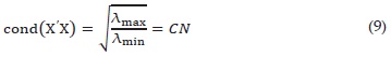
Small values of λ_mín and large values of λ_máx indicate the presence of collinearity. Low values of the condition number indicate some level of stability or conditioning in the least squares estimate.

We propose as a criterion for selection of the slack variable the SV_xq model with the smallest CN value.

Suppose the case where there are only three components: x₁, x₂, x₃. Here we would want to determine which component should be used as slack variable. When we have three components we can fit three different SV models, this is, we can fit the SV model using x₁ as a slack variable (SV_x1), or use x₂ as a slack variable (SV_x2) or use x₃ (SV_x3). These three SV models have the form

SV_x1 = γ₀ + γ₂x₂ + γ₃x₃

SV_x2 = γ₀ + γ₁x₁ + γ₃x₃

SV_x3 = γ₀ + γ₁x₁ + γ₃x₃

Thus, we can calculate the CN (9) to each of the three models, and for example, if SV x₁ has the minimum CN that mean that x₁ is the component that have to be use as a slack variable.

In assessing the conditioning of information matrix for estimating the parameters in a regression model, assessment of the variance inflation factors associated with the regression coefficients of the X' X matrix, is widely used method.

The variance inflation factor (VIF) associated with the estimated regression coefficients γ_j is given by

To evaluate the overall collinearity level of a model, we propose the mean variance inflation factor (MVIF),

Following are four numerical examples:

Example 1

Piepel (2009) use an artificial example involving mixtures of two drugs (x₁ and x₂), an enhancer (x₃), and a filler (x₄), where

An 18-point, face-centered cube was used as the design, which contains 8 factorial points, 6 face centroids, and 4 center point replicates. The experimental design points and values of the response variable are listed in Table 1.

Listed below are the CN values for the four quadratic SV models using (9) and the data in Table 1.

According to the proposed criterion x₄ should be used as a slack variable.

Table 3 shows that the VIFs for the SV_x4 are generally considerably smaller than those for the SV_x1, SV_x2 and SV_x3. The MVIF for the SV_x4, is less that of the SV_x1, SV_x2 and SV_x3 as well, indicating a more stable analysis.

Example 2

Prescott (2002) described an experiment to study the effects of different mixtures in which

The 13-Points Optimal Design is provided in Table 4.

Listed below are the CN values for the four quadratic SV models using (9) and the data in Table 5.

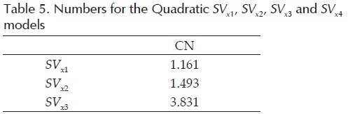
According to the proposed criterion should be used as a slack variable ( Table 6).

The VIFs for the SV_x1 are generally considerably smaller than those for the SV_x2 and SV_x3. The MVIF for the SV_x1, is less that of the SV_x2 and SV_x3, indicating a more stable analysis.

 

Example 3

Cornell (2000) describes a study where the solubility of butoconazole nitrate, an anti-fungal agent, was studied as a function of the proportions of the co-solvents polyethylene glycol 400 (x₁), glycerin (x₂), polysor polysorbate 60 (x₃), along with water (x₄). Constraints on the component proportions were

A 10-point D-optimal design was selected for fitting a quadratic model. The design consisted of 6 of the 10 extreme vertices and midpoints of 4 of the edges of the constraints region. Listed in Table 7 are the coordinates of the components and the solubility values ranging in magnitude from 3.4 to 12.4 mg/ml.

Listed below are the CN values for the four quadratic SV models using (9) and the data in Table 8.

According to the proposed criterion x₄ should be used as a slack variable (Table 9).

The VIFs for the SV_x4 are generally considerably smaller than those for the SV_x1 -, SV_x2 and SV_x3. The MVIF for the SV_x4, is also less that of the SV_x1, SV_x2 and SV_x3 indicating a more stable analysis.

Example 4

Cornell and Gorman (2003) describe a study involving three components and seven design points in the reduced region constrained by the inequalities

The data for the example are reproduced in Table 10 below

Listed below are the CN values for the four quadratic SV models using (9) and the data in Table 11.

According to the proposed criterion x₂ should be used as a slack variable (Table 12).

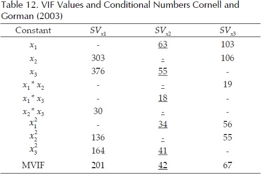
The VIFs for the SV_x2 are generally considerably smaller than those for the SV_x1 and SV_x2. The MVIF for the SV_x2, is less that of the SV_x1 and SV_x3, indicating a more stable analysis.

 

Linear transformations

Thirty two years ago, Gorman (1970) pointed out that fitting polynomials to mixture data by linear least squares often leads to inaccurate computer solutions when are restraints on composition. By restraints on composition, he meant that data are collected from a highly constrained region inside the mixture simplex. As illustrated by Prescott and Draper (2009) if the design space is restricted to a reduced region within the simplex, and these models are fitted in terms of the original x₁ variables, the estimated coefficients might bear little resemblance to the magnitudes of the actual observations, because they are extrapolated out to the full simplex. The coefficients may be many times greater (in absolute value) than the observations, which some practitioners find disconcerting ( Cornell and Gorman, 2003).

Snee and Rayner (1982) proposed alternative models to the Scheffe model in the original component proportion when the data are collected from a highly constrained mixture region. Montgomery and Voth (1994) discussed ways of overcoming high leverage points and collinearity by replicating the high leverage points and imposing other design considerations to combat collinearity. Cornell and Gorman (2003) introduce two new mixture model forms, these models not removing the collinearity on the coefficient estimates, but diminish its influence. Prescott and Draper (2009) introduce a different alternative transformation that identifies the largest simplex-shaped space contained within the restricted region.

In this section, we introduce two alternative transformations for the SV-model, which make the SV-model a better conditioned model.

The first alternative transformation for the SV-model is given by

where mín and máx are the minimum and maximum value of x_i.

We consider the example 2 used in section 3 (Prescott et al., 2002).

Table 13 shows the analysis of the SV fitted model when applied to the original data without the application of any transformations.

As we saw above, the VIFs and MVIF for the X' X matrices using original data are quite high. On the other hand, comparing the range of the y-values in Table 4 (Section 3) with the fitted model coefficients in Table 13, we see that they bear little resemblance to one another because the coefficients represent estimates well outside the region of the data.

To ameliorate this, we applied (12) to the data in Table 4 (Section 3). Table 14 shows the date in transformed units x_i'.

Table 15 shows the analysis of the SV fitted model when applied to the transformed units (x_i').

As can be seen in Table 15, the transformation resulted in coefficients smaller than those in the models shown in Table 13 (data without transformation). This transformation provides a nice compromise, producing coefficients of size similar to the observations. In the same way the value of MVIF reduced.

The second alternative transformation for the SV-model is given by

where mín and máx are the minimum and maximum value of x_i.

For the second alternative transformation we consider the same example that was used in the first alternative transformation Prescott et al.(2002). Table 16 shows the date in transformed units x_i".

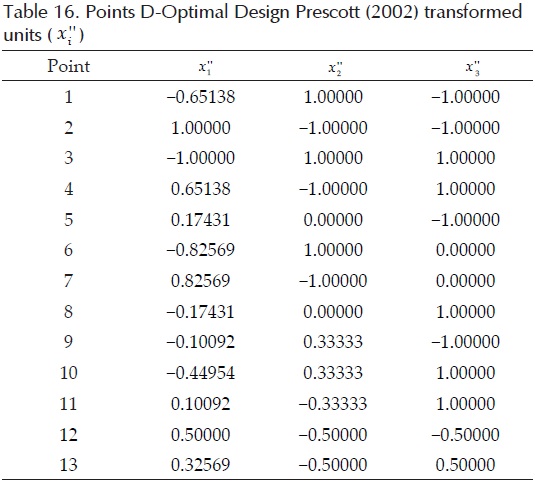
Table 17 shows the analysis of the SV fitted model when applied to the transformed units (x_i").

As can be seen in Table 17 the second transformation appears to go too far, producing coefficients that are generally smaller than the observations. However, the values of the VIFs and the MVIF are considerably lower than those shown in Table 15.

 

Conclusions

In this paper, we study the properties of the SV-model. Based on our study, we would recommend the practitioners to use the slack variable approach. While using the SV-model, we can choose slack variable using criterion proposed in Section 3. Reasonable transformation should be used on the design to improve the numerical stability.

Improvement in the conditioning of the information matrix generally reduces the variances of individual estimated regression coefficients, reduces the correlation between the estimators, and makes the model less dependent on the precise location of the design points. Although a badly conditioned fit can still provide useful contour information, practitioners are more comfortable with better-conditioned, stable models.

We strongly recommend to practitioners consider the relationship between SV-model and S-model in order to avoid misleading results and conclusion.

 

References

Cain M. and Price M.L.R. Optimal Mixture Design. Applied Statistics, volumen 35, 1986:1-7.         [ Links ]

Cornell J.A. Fitting a slack-sariable model to mixture data: some questions raised. Journal of Quality Technology, volumen 32, 2000: 133-47.         [ Links ]

Cornell J.A. Experiments with mixtures: designs, models and the analysis of mixture data, 3rd ed., New York, John Wiley and Sons, 2002, 333-337.         [ Links ]

Cornell J.A., Gorman J.W. Two new mixture models: living with collinearity but removing its influence. Journal of Quality Technology, volumen 35, 2003: 78-88.         [ Links ]

Draper N.R. and Pukelsheim J. Mixture models based on homogenous polynomials. Journal of Statistical Planning and Inference, volumen 71, 1998: 303-311.         [ Links ]

Fonner D.E., Buck J.R., Banker G.S. Mathematical optimization techniques in drug product design and process analysis. Journal of Pharmaceutical Sciences, volumen 59, 1970: 1587-1596.         [ Links ]

Gorman J.W. Fitting equations to mixture data with restraints on composition. Journal of Quality Technology, volumen 2, 1970: 186-194.         [ Links ]

Goldfarb H.B., Anderson-Cook C.M., Borror C.M., Montgomery D.C. Fraction of design space plots for assessing mixture and mixture-process designs. Journal of Quality Technology, volumen 36, 2004: 169-79.         [ Links ]

Ralph C., John St. Experiments with mixtures, ill-conditioning, and ridge regression. Journal of Quality Technology, volumen 16, 1984: 81-96.         [ Links ]

Khuri A.I. Slack-variable models versus scheffés mixture models. Journal of Applied Statistics, volumen 32, 2005: 887-908.         [ Links ]

Kowalski S.M., Cornell J.A., Vining G.G. Split-plot designs and estimation methods for mixture experiments with process variables. Technometrics, volumen 44, 2002: 72-79.         [ Links ]

Landmesser S.M. and Piepel G.F. Comparison of slack variable and mixture experiment approaches. Proceedings of the Joint Statistical Meetings, 2007: 1711-7.         [ Links ]

Snee R.D. Marquardt D.W. Test statistics for mixture models. Technometrics, volumen 16, 1974: 533-7.         [ Links ]

Montgomery D.C. and Voth S. R. Multicollinearity and leverage in mixture experiments. Journal of Quality Technology, volumen 26, (issue 2), 1994.         [ Links ]

Myers R.H., Montgomery D.C., Anderson-Cook C.M. Response surface methodology: process optimization using designed experiments, 3rd ed., New York, John Wiley and Sons, 2009, 219-264.         [ Links ]

Prescott P., Dean A.M., Draper N.R., Lewis S.M. Mixture experiments: ill-conditioning and quadratic model specificatión. Technometrics, volumen 44, 2002: 260-8.         [ Links ]

Prescott P. and Draper N.R. Modeling in restricted mixture experiment spaces for three mixture components. Quality Technology and Quantitative Management, volumen 6, 2009: 207-17.         [ Links ]

Piepel G.F. and Cornell J.A. Mixture experiment approaches: examples, discussion, and recommendations. Journal of Quality Technology, volumen 26, 1994: 177-96.         [ Links ]

Piepel G.F. and Cornell J. A. Models for mixture experiments when the response depends on the total amount. Technometrics, volumen 27, 1985: 219-27.         [ Links ]

Piepel G.F. and Landmesser S.M. Mixture experiment alternatives to the slack variable approach. Quality Engineering, volumen 21, 2009: 262-76.         [ Links ]

Scheffe H. Experiments with mixtures. Journal of the Royal Statistical Society, Series B, volumen 20, 1958: 344-60.         [ Links ]

Snee R.D. Techniques for the analysis of mixture data. Technometrics, volumen 15, 1973: 517-28.         [ Links ]

Snee R.D. and Rayner A.A. Assessing the accuracy of mixture model regression calculations. Journal of Quality Technology, volumen 14, 1982: 67-79.         [ Links ]

Soo H.M., Sander E.H., Kess D.W. Definition of a prediction model for determination of the effect of processing and compositional parameters on the textural characteristics of fabricated shrimp. Journal of Food Science, volumen 43, 1978: 1165-1171.         [ Links ]

 

Citation for this article:

Chicago style citation
Cruz-Salgado, Javier. Selecting the slack variable in mixture experiment. Ingeniería Investigación y Tecnología, XVI, 04 (2015): 613-623.

ISO 690 citation style
Cruz-Salgado J. Selecting the slack variable in mixture experiment. Ingeniería Investigación y Tecnología, volume XVI (issue 4), October-December 2015: 613-623.

 

About the author

Javier Cruz-Salgado. BS, Industrial Engineering, Universidad Tecnológica de León, March 2007. MS, Manufacturing and Industrial Engineering, CIATEC/CONACYT, August 2012. PhD Student, Manufacturing and Industrial Engineering, CIATEC/CONACYT. Intern at Materials Research Department CIATEC 2011-2012. Research stay at Illinois Institute of Technology in the Department of Applied Matheh matics 2013.