


Serviços Personalizados
Journal
Artigo
 Inglês (pdf)
 Artigo em XML
 Referências do artigo
 Enviar este artigo por email
Indicadores
-
 Citado por SciELO
 -
 Acessos
Links relacionados
-
 Similares em
SciELO
Similares em
SciELO
Compartilhar

 Permalink
Ingeniería, investigación y tecnología
versão On-line ISSN 2594-0732versão impressa ISSN 1405-7743
Ing. invest. y tecnol. vol.15 no.3 Ciudad de México Jul./Set. 2014
Ground-Wave Propagation Effects on Transmission Lines through Error Images
Efectos de la propagación de ondas en tierra en líneas de transmisión a través de imágenes de error
Uribe-Campos Felipe Alejandro
Departamento de Mecánica Eléctrica, División de Ingenierías Universidad de Guadalajara, CUCEI. Correo: fauribe@ieee.org
Received: March 2013,
Reevaluated: April 2013,
Accepted: June 2013
Abstract
Electromagnetic transient calculation of overhead transmission lines is strongly influenced by the natural resistivity of the ground. This varies from 1-10K (Ω·m) depending on several media factors and on the physical composition of the ground. The accuracy on the calculation of a system transient response depends in part in the ground return model, which should consider the line geometry, the electrical resistivity and the frequency dependence of the power source. Up to date, there are only a few reports on the specialized literature about analyzing the effects produced by the presence of an imperfectly conducting ground of transmission lines in a transient state. A broad range analysis of three of the most often used ground-return models for calculating electromagnetic transients of overhead transmission lines is performed in this paper. The behavior of modal propagation in ground is analyzed here into effects of first and second order. Finally, a numerical tool based on relative error images is proposed in this paper as an aid for the analyst engineer to estimate the incurred error by using approximate ground-return models when calculating transients of overhead transmission lines.
Keywords: ground-return effects, earth impedances, low frequency effects, electromagnetic transients, error images.
Resumen
El cálculo de transitorios electromagnéticos en líneas aéreas de transmisión está fuertemente influenciado por la resistividad natural eléctrica del suelo. Esta puede variar de 1-10K (Ω·m) dependiendo de diversos factores en el medio y de la composición física del suelo. La precisión en el cálculo de la respuesta transitoria en un sistema depende en parte del modelo de retorno por tierra, el cual debe considerar la geometría de la línea, la resistividad eléctrica y la dependencia frecuencial de la fuente de alimentación. Hasta la fecha hay pocos reportes en la literatura especializada acerca del análisis de los efectos producidos por la presencia de un suelo conductor imperfecto de líneas de transmisión en estado transitorio. En este artículo se realiza un análisis de amplio rango a tres de los modelos de tierra actualmente más utilizados para cálculo de transitorios electromagnéticos en líneas aéreas de transmisión. El comportamiento de la propagación modal en tierra se analiza aquí en dos tipos de efectos de retorno por tierra. Finalmente, se propone en este artículo una herramienta numérica basada en imágenes de error relativo como una ayuda para que el ingeniero analista pueda estimar el error incurrido por utilizar modelos aproximados de tierra para el cálculo de transitorios en líneas aéreas de transmisión.
Descriptores: efectos de retorno por tierra, impedancias de tierra, efectos de baja frecuencia, transitorios electromagnéticos, imágenes de error.
Introduction
The analysis of wave propagation effects on overhead transmission systems due to the presence of an imperfectly conducting ground, is critically important to assess the frequency dependent losses and phase delay of ground modes. By its own structure, the electric line parameters Z (series-impedance) and γ (shunt-admittance) characterize the ground-return effects on a first and second order, respectively.
First order effects arise when the influence of the ground prevails over the geometric influence of the line. This is the case when the characteristic impedance of the system,  , plays an important role in the simulation; e. g., on transient short-circuit currents calculation (Marti and Uribe, 2002). In this case, the frequency dependence of ZC is entirely due to the ground-return path (Wedepohl, 1965).
The second order effects arise in the calculation of the modal voltage propagation function of the lin e –γ·λ where  and l is the line length. In terms of propagation functions, when forming the product Z×ϒ the geometric effects tend to cancel out each other, except for the different influence of the ground (Marti and Uribe, 2002).
The problem here is that, up-to-date, there is no general criterion to evaluate the ground conduction effects on transmission line propagation. Another problem is the evaluation of how the ground-return conduction effects impact on transmission line systems when switching transients occur.
Thus, it is the main idea of this paper to perform a new algorithmic methodology to analyze the first and second order ground-return conduction effects on voltage and current transient waveforms of overhead transmission systems.
First, a broad range solution of the Carson's integral (Carson, 1926) is developed and implemented in this paper based on a previously established algorithmic technique published in (Uribe et al., 2004; Ramirez and Uribe, 2007). In addition, normalized dimensionless parameter comparisons with the Carson's series and complex-depth closed-form approximations (Gari, 1976; Kostenko, 1955; Deri et al., 1981; Alvarado and Betancourt, 1983) are obtained here through the relative error criterion. This methodology yields a new technique proposed here as an aid to estimate ground-return modeling error on transients calculation through error images.
Finally, the impact of ground-return modeling errors on transients calculation is identified here with an application example accurately solved via the Numerical Laplace Transform (Uribe et al., 2002).
Algorithmic solution of Carson's integral
Figure 1 shows two overhead infinite thin perfect conductors over an imperfectly conducting ground 0 < σ2 < ∞. The series-impedances contribution (in Ω∙m) is given by (Marti and Uribe, 2002).
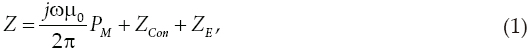
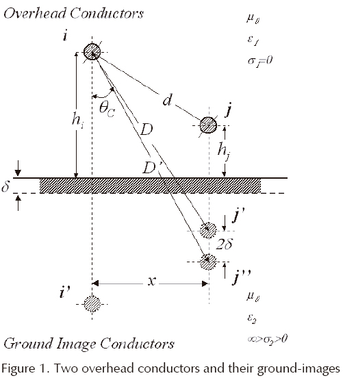
where PM is the dimension less Maxwell's potential-coefficient, ZCon is the internal conductor impedance and ZE introduces the ground-return impedance contribution. Assuming a uniform line, homogeneous soil and neglecting inner displacement currents, the self or mutual ground-return impedances are given by the Carson's integral (in MKS system) (Carson, 1926)

where
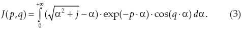
A characterization of the Carson's dimensionless parameters p and q is useful to analyze the regular oscillating pattern of the integrand where α is the dummy variable. Carson introduced in (Carson, 1926) the following physical variables of the medium properties according to Figure 1:
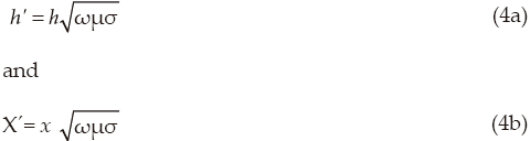
Expression (4a) and (4b) are normalized by the magnitude of the Skin Effect (Marti and Uribe, 2002; Wedepohl, 1965; Carson, 1926; Uribe et al., 2004; Ramírez and Uribe, 2007; Gari, 1976; Kostenko, 1955; Deri et al., 1981; Alvarado and Betancourt, 1983; Uribe et al., 2002; Piessens et al., 1983; Using MATLAB, 2011; Dommel, 1986). Now, Carson's dimensionless parameter p and q for the self-impedance case are given by

and for mutual impedances:

The integrand in (3) contains three factors. The first two are of the damping type while the third is regular oscillatory. The pattern of these factors suggests a new strategy for its numerical efficient solution. Consider the solution of the first factor radical function in (3) as (Uribe et al., 2004; Ramirez and Uribe, 2007)
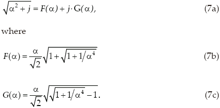
Functions F(α) and G(α) provide the additional damping components to the integrand. Substituting (7b) and (7c) in (3) and decomposing into real and imaginary components, (3) becomes

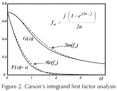
Functions F(α) – α and G(α) in the first complex factor of (8) are monotonically decreasing. Figure 2 illustrates the behavior of these functions that for α > 1 1tends asymptotically to "1/(8α3)" and "1/(2α)", respectively (Uribe et al., 2004; Ramirez and Uribe, 2007).
The second complex factor in (8) only depends on the normalized parameter p. This factor is a pure damping exponential function. The truncation criterion developed in (Uribe et al., 2004; Ramirez and Uribe, 2007) with a relative error control can be extracted from its properties as

and the truncating criterion by approximating "J(p,q)" for the new truncated range would be (Uribe et al., 2004; Ramírez and Uribe, 2007)

The error level can be controlled refining λ. A value of λ = 10 has proved satisfactory enough for many practical application cases.
The third factor in (8) provides regular oscillations to the integrand which increases equal times as the argument q×α exceeds the value of π/2. This argument is related to the horizontal distance between conductors (x in Figure1) and to the magnitude of Skin Effect Layer Thickness (Carson, 1926; Uribe et al., 2004; Ramírez and Uribe, 2007). Within the range [0, αmax] this factor will not oscillate if

If condition (11a) is not satisfied, the integrand oscillations would produce magnified round-off errors when integrating with generic quadrature routines (Piessens et al., 1983). To avoid this problem, it is necessary to detect the zero crossings with:
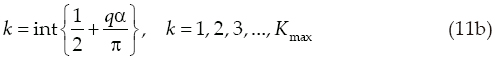
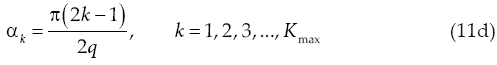
where k is the corresponding oscillation sequence, "int" is the complete integer value and Kmax indicates the maximum number of oscillations that are given by

Notice in (11c) that (q/p) = (x'/h'). Obviously, from (11b) for each value of k the integrand zero crossing would be
A new reliable and efficient broad range algorithmic evaluation of the Carson's integral has been obtained by using the truncating criterion in (10) with the zero crossing identification in (11) for 10 × 532 samples inside Table 1 ranges (Uribe et al., 2004; Ramirez and Uribe, 2007).

The physical variable ranges in Table 1 have been used to calculate the normalized Carson parameters shown in Table 2 to perform the algorithmic calculation of (8).

Figures 3a and 3b depict the broad solution set obtained with the algorithmic technique proposed in this paper.
The figures were generated solving Carson's integral 10 × 532 timeswhich takes about more than one second on a 3.4GHz, 8GB RAM computer, running MATLAB® V. 7.12 (Using MATLAB®, 2001).
Implementation of Carson's series and complex depth formulae
In the synthesis of frequency dependent electromagnetic transients the need of a higher sampling refinement interval is often required (Wedepohl, 1965; Uribe et al., 2002). There are cases when it is necessary to handle very small or high ground conductivity values; e.g., from rocky to moist ground (Dommel, 1986). Also there are other cases when the distance between conductors is wider (θC > π/4); e.g., interference on communication lines due to a power line fault (Dommel, 1986). In all these cases, it is highly convenient to have an accurate methodology for calculating the mutual ground-return impedances between both energy systems.
A numerical version of the Carson's series has been also implemented here to test and verify the efficiency and accuracy of the algorithmic solution proposed in this paper (Carson, 1926; Dommel, 1986). However, in the treated application case, the series solution presented some serious disadvantages; the number of terms is practically unpredictable, numerical discontinuities emerges when switching from infinite to finite convergence ranges and also, it turns time consuming. For these reasons, the original series solution in Carson (1926) cannot be used to generate the error images proposed in the following paper section.
Thus, using the original Carson's parameters the following normalized distance according to Figure 1 is introduced as (Carson, 1926)

with a Carson's angle between vectors of

Regarding the component partition (8), one can infer that

and according to this paper nomenclature
The following Carson parameter introduces the normalized distance between a real conductor in the air and the image of the other conductor inside the ground. This parameter also was used as a boundary quantity to adjust the switching process of the series when changing from a finite range a ≤ 5 into an infinite one a > 5 (Carson, 1926; Dommel, 1986):

As an application example, consider an aerial transmission line with conductor height h = 20 m. The distance between conductors is 0 ≤ x ≤ 1 Km. The ground conductivity is 0.01 S/m and the frequency range is 1 ≤ ω/2π ≤ 106 Hz.
To test accuracy and efficiency of the here developed algorithmic technique, an equivalent solution of J(p,q) in (12c) has been calculated using the Carson series (Carson, 1926). The real and imaginary components are shown in Figure 4. At first sight the differences appear to be indistinguishable, but in Figure 5, two types of numeric discontinuities arise when calculating the relative error (Ramirez and Uribe, 2007).
The first one is due to the series adjustment, while the second (in the form of peak discontinuities) is due to the switching series process, when changing from an infinite range into the new truncated range (Dommel, 1986).
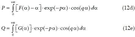
For this example layout, Figure 6 shows the magnitude and angle relationship between the vector components P and Q from (12d, e) calculated with the Carson series varying parameter D. The here obtained curves match with the obtained ones in Carson's paper confirming the accuracy of the method (Carson, 1926).
In addition, the obtained algorithmic solution set is used to confirm the accuracy ranges of the complex-depth based formulas of Gary (1976), Kostenko (1955), Deri et al. (1981)and Alvarado et al. (1983).
Basically, classical images complex depth formulas are based in the following expression
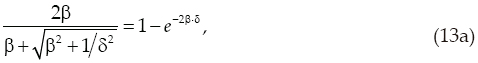
where  . After some algebraic manipulations (13a) is transformed into (Ramirez and Uribe, 2007)

The behavior of F(α) and G(α) is shown in Figure 2, as well as for ƒn. On introducing the right side of (13b) into (8) we have

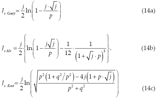
An analytical solution can be obtained directly from (13c) (Gary, 1976; Kostenko, 1955; Deri et al., 1981; Alvarado et al., 1983). Now, the complex depth formulae are transformed into a normalized dimensionless parameter expression of p and q. Thus, according to ZE in (2) the self-impedance Js and the mutual-impedance Jm for the Gary, Kostenko, Deri et. al., and Alvarado et. al. formulae becomes
And for the mutual impedance case
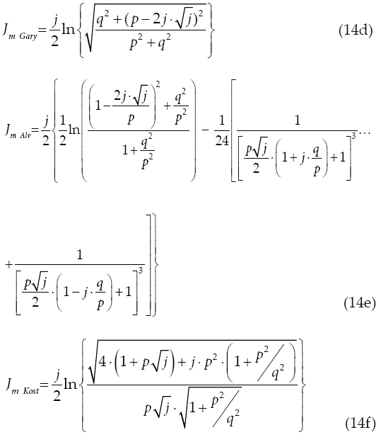
The approximation (14) for self or mutual ZE in (2), substitutes J(p,q) in (8). In essence Gary, Kostenko, Deri et al. formulas have presented almost identical behavior between each other when plotting their error images. In consequence, only the images formed with the Gary and Alvarado et al. expressions are the only ones studied in this paper. Thus, the broad range result set is used now to generate the curves shown in Figure 7 for the P and Q components of (12c) in a parametric version of (14d) and (14e).
Error images estimation of ground models
The ground resistivity magnitude is introduced here into the electromagnetic transient calculation via the ZE model. Thus, an important problem arises when estimating the ground modeling error. A new technique to estimate ground modeling errors on electromagnetic transient calculation is proposed in this paper section through error images. First, the broad range algorithmic solution (8), the approximated formulas by Gary in (14d) and the one by Alvarado et al. in (14e) are compared here through the relative error criterion as (Uribe et al., 2004; Ramirez and Uribe, 2007)

where ZE is the algorithmic solution ground impedance and ZE, Approx, Approx is the approximate images ground impedance formula. Figure 8 shows the generated error images (15a) using 102 samples inside data in Table 2. Each image shows five error regions. The error levels lie in the range of 1% ≤ εrel ≤ 10%.
Thus, a practical ground-modeling error estimation algorithm through images is proposed as follows:
First step. Using physical variables (hi, hj, x, r) and relative medium properties (μr, σ, εr), evaluate the parameter relation q/p for each voltage coupling loop inside the system. The larger number of circuit loops, the more error line paths images are generated.
Second step. Calculate the NLT parameters (Uribe et al., 2002). Set the observation time Tobs and the number of samples Nsamo, then the other parameters can be calculated as

where ω is the angular frequency, Δt is the sampled time increment, Ω is the truncating frequency, Δω is the sampled frequency increment, c is the complex frequency damping coefficient and n is the discretization relative error level. Further, evaluate the complex frequency variable

Third step. Find the maxima and minima boundary values of the transient Skin Effect variable using (15f) for calculating δ

then, evaluate the normalized function pmax/min as

Fourth step. Plot the previously generated error image for the ground-model and trace the error line paths according q/p sorting min and max frequency samples.
Fifth step. Check the sampled error points region in the images. Their influence area would be their corresponding error levels.
Ground-return conduction effects in transients
In this research paper, the ground-return effects are analyzed according to a first and second order kind. On one hand, first order effects are given when the influence of the ground prevails over the geometric influence of the line. This is the case when ZC has an important role in the numerical simulation. In the frequency limits ZC becomes

The frequency dependency of (16a) is entirely due to the ground-return contribution, since ZCon → 0.
On the other hand, the second order effects arise when forming the product Z·ϒ, because the geometric effects tend to cancel out each other, except for the different influence of the ground (Marti, 2002).
This is the case of the voltage propagation function e–ϒxlg×l. Thus, ϒ tends asymptotically to
where U is the unit matrix (Wedepohl, 1965).
Consider a typical overhead transmission system as the one depicted in Figure 9. This is a homogeneous three-phase power line with a ground wire and a single communications line sharing a common right of way. The system length is 10 Km. The corresponding conductors radii are ri= 3.20 cm, rj= 2.5 cm and rk = 1.5 cm. The soil conductivity is σ = 0.005 S/m.
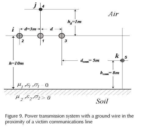
The frequency dependent behavior of modal propagation functions ZC and e–ϒ·l for each numbered conductor in Figure 9 is illustrated in Figure 10. The impact of Gary and Alvarado ground-return models (Gary, 1976; Kostenko, 1955; Deri et al., 1981; Alvarado et al., 1983) in the transient step response is illustrated here the by means of a two circuit test using the NLT for the energy system shown in Figure 9 (Uribe et al., 2002).
The first test is the calculation of the transient step voltage-response at the remote end with an open circuit condition of the system using the here treated ground-return models for comparison.
Figures 11a and 11b show the receiving end voltage response at the energized conductor (No. 1 in Figure 9) and the induced voltage response at the communications line (No. 5 in Figure 9), respectively.
Figure 11c and 11d show the corresponding relative errors (15a) calculated for the obtained voltages, for the Gary and Alvarado-Betancourt models with respect to the Carson solution (Gary, 1976; Kostenko, 1955; Deri et al., 1981; Alvarado et al., 1983). In this case the Gary model is amazingly accurate.
The second test consists in the calculation of the transient step current response at the remote end with a short circuit condition of the system calculated with the here treated approximated ground-return models.
Figure 12a show the current transient step response calculated at the energized conductor (No. 1), while Figure 12b depicts the corresponding circulating current at the victim circuit of communications line (No. 5).
Figures 12c and 12d, show the calculated relative errors (15a) for the circulating currents at the energized conductor and at the induced communications line, respectively. One more time the accuracy of the Gary model can be noticed from these figures.
As ground-return models are strong frequency dependent as can be seen in Figure 10b, a better general tool for analyzing the effects of a ground-return model in electromagnetic transients calculation is the images methodology proposed in Figure 13.
Consider the error images in Figure 8 calculated in magnitude quantities for the Deri et al.(1981) and Alvarado et al. (1983)models. Two sets of error line paths have been traced in each of both figures. The horizontal error line path, represents a particular coupling circuit loop for any set of two specific conductors present in the transmission system shown in Figure 9.
As an application example, consider the two sets of traced error line paths shown in Figure 13. The first set p1-p2 and p5-p6 corresponds to the loop formed between the energized power conductor and the victim communications line.
The second set of error line paths p3-p4 and p7-p8 correspond to the hypothetical case of calculating four times the magnitude q/p. An error less than 1% corresponds to the image points p5 and p7, which have an implicit frequency of 220 Hz. The error of p6 lies well within 1% and 2%. Points p1, p2 and p3 have an error between 4% and 6%. The image points p4 and p8 lie into region five, having an error greater than 10%. In this application case, any other image point has an implicit truncating frequency of 102 KHz.
Conclusions
An accurate numerical algorithm for solving the Carson's integral, their classical series expansion and complex-depth approximate formulae, has been implemented in this paper for a broad range of applications, emphasizing the case θC > π/2.
In the specific application example presented in this paper the transient-step responses calculated at the remote end of open-circuit voltages and short-circuit circulating currents, the ground-return model of Gary presented a more accurate result than the Alvarado et al. model. The main differences are probably due to the validity ranges of the implicit frequency in the transient calculation and, of the separation distance between conductors of the latter model.
A new technique for estimating ground-return modeling errors on electromagnetic transients calculation is proposed in this paper through error images.
The frequency dependence of the ground has been separated here into effects of first and second order. These are mainly due to the modal propagation functions in the ground ϒ(ω) and to the characteristic impedance function ZC(ω).
A methodology to analyze the impact of ground modeling errors on low frequency transients has been proposed here through error images, tracing simple error line paths on each image for a certain ground model having a universal applicability.

References
Alvarado F., Betancourt R. An Accurate Closed-Form Approx. For Ground Return Impedance Calculations. Proc.of the IEEE, volume 71 (issue 2), 1983: 279-280. [ Links ]
Carson J.R. Wave propagation in overhead wires with ground return. Bell Systems Tech. J., 1926: 539-554. [ Links ]
Deri A., Tevan G., Semlyen A. and Castanheira A. The Complex Ground Return Plane: a Simplified Model for Homogeneous and Multi-Layer Earth Return. IEEE Transactions on Power Apparatus and Systems, volume PAS-100 (issue 8), August 1981: 3686-3693. [ Links ]
Dommel W. Electromagnetic Transients Program Reference Manual (EMTP Theory Book), Prepared for Bonneville Power Administration, P.O. Box 3621, Portland, Ore., 97208, USA, 1986. [ Links ]
Gary C. Approche Complete de la Propagation Multifilaire en Haute Frequence par Utilisation des Matrices Complexes. E.D.F Bulletin de la Direction des Etudes et Recherches, serie B, (issues 3/4), 1976 : 5-20. [ Links ]
Kostenko M.V. Mutual Impedance of Earth-Return Overhead Lines Taking into Account the Skin-Effect. Elektritchestvo, (issue 10), 1955: 29-34. [ Links ]
Marti J.R. Thesis Report Uribe F.A. Algorithmic Evaluation of Pollaczek Integral and its Application to EM Transient Analysis of Underground Transmission Systems, (Ph.D. dissertation), Dept. Electrical. Eng., Cinvestav, Unidad Guadalajara, Jalisco, November 2002. [ Links ]
Piessens R., Doncker E., Ueberhuber C.W., Kahaner D.K. Quad Pack- A Subroutine Package for Automatic Integration, Springer-Verlag, Berlin Heidelberg, New York Tokyo, 1983. [ Links ]
Ramirez A. and Uribe F. A Broad Range Algorithm for the Evaluation of Carson's Integral. IEEE Trans. on Pow. Del., volume 22 (issue 2), 2007: 1188-1193. [ Links ]
Uribe F.A., Naredo J.L., Moreno P. and Guardado L. Algorithmic Evaluation of Underground Cable Earth Impedances. IEEE Transactions on Power Delivery, volume 19 (issue 1), January 2004: 316-322. [ Links ]
Uribe F.A., Naredo J.L., Moreno P. and Guardado L. Electromagnetic Transients in Underground Transmission Systems Trough The Numerical Laplace Transform. Elsevier Science Ltd, Electrical Power and Energy Systems, volume 24, 2002: 215-221. [ Links ]
Using MATLAB, Matrix-Laboratory, The Math Works Inc., Natick, MA, Matlab-7.12 (R2011a). [ Links ]
Wedepohl L.M. Electrical Characteristics of Polyphase Transmission Systems with Special Reference to Boundary-Value Calculations at Power-Line Carrier Frequencies. Proceedings of the IEE, volume 112 (isuue 11), November 1965. [ Links ]
About the author
Felipe Alejandro Uribe-Campos. Received the B.Sc. and M.Sc. degrees of Electrical Engineering, both from the State University of Guadalajara, in 1994 and 1998, respectively. During 2001 he was a visiting researcher at the University of British Columbia, B.C. Canada. In 2002 he received the Dr.Sc. degree in Electrical Engineering from the Center for Research and Advanced Studies of Mexico. The dissertation was awarded with the Arturo Rosenblueth prize. From 2003 to 2006 he was a full professor with the Electrical Graduate Program at the state University of Nuevo Leon, México. From May 2006, he joined the Electrical Engineering Graduate Program at the State University of Guadalajara, México, where he is currently a full time researcher. Since 2004, he is a member of the Mexico's National System of Researchers (SNI). His primary interest is the electromagnetic simulation of biological tissues for early cancer detection and power system harmonic and transient analysis.

