Exponential Convergence of Multiquadric Collocation Method: a Numerical Study

 

Convergencia exponencial del esquema de colocación con multicuádricos: un estudio numérico

 

J.A. Muñoz–Gómez¹, P. González–Casanova² and G. Rodríguez–Gómez³

 

¹ Departamento de Ingenierías, CUCSUR. Universidad de Guadalajara, Autlán, Jalisco, México. E–mail: jose.munoz@cucsur.udg.mx

² UICA–DGSCA, Universidad Nacional Autónoma de México. E–mail: pedrogc@dgsca2.unam.mx

³ Ciencias Computacionales. Instituto Nacional de Astrofísica, Óptica y Electrónica, Puebla, México. E–mail: grodrig@inaoep.mx

 

Recibido: noviembre de 2006
Aceptado: noviembre de 2008

 

Abstract

Recent numerical studies have proved that multiquadric collocation methods can achieve exponential rate of convergence for elliptic problems. Although some investigations has been performed for time dependent problems, the influence of the shape parameter of the multiquadric kernel on the convergence rate of these schemes has not been studied. In this article, we investigate this issue and the influence of the Péclet number on the rate of convergence for a convection diffusion problem by using both an explicit and implicit multiquadric collocation techniques. We found that for low to moderate Péclet number an exponential rate of convergence can be attained. In addition, we found that increasing the value of the Péclet number produces a value reduction of the coefficient that determines the exponential rate of convergence. More over, we numerically showed that the optimal value of the shape parameter decreases monotonically when the diffusive coefficient is reduced.

Keywords: Radial basis functions, multiquadric, convection–diffusion, partial differential equation.

 

Resumen

Experimentos numéricos recientes sobre los métodos de colocación con mulitcuádricos han demostrado que éstos pueden alcanzar razones de convergencia exponencial en problemas de tipo elípticos. Si bien, algunas investigaciones se han realizado para problemas dependientes del tiempo, la influencia del parámetro c del núcleo multicuádrico en la razón de convergencia de éstos esquemas no ha sido estudiada. En la presente investigación se analiza este tópico y la influencia del número de Péclet en la razón de convergencia para un problema convectivo difusivo, considerando un esquema de discretización implícito y explicito con técnicas de colocación con mulitcuádricos. Demostramos numéricamente que para valores bajos a moderados del coeficiente de Péclet se obtiene una razón de convergencia exponencial. Además, encontramos que al aumentar el número de Péclet origina una reducción en valor del coeficiente que determina la razón de convergencia exponencial. Adicionalmente, determinamos que el valor óptimo del parámetro c decrece monótonicamente cuando el coeficiente difusivo es disminuido.

Desciptores: Funciones de base radial, multicuádrico, convección–difusión, ecuación diferencial parcial.

 

Introduction

It is well known that within the study of the numerical multiquadric unsymmetric collocation methods for partial differential equations (Kansa, 1990), a major problem is the determination of the shape parameter. Several authors have avoided the use of this radial basis function due to this difficulty, see; (Boztosun et al., 2002; Zerroukat et al., 2000; Li et al., 2003). Some recent studies has been done to investigate this problem, (Fornberg et al., 2004; Larsson et al., 2005). In particular (Cheng et al., 2003), has treated an elliptic problem showing that an exponential rate of convergence can be attained for h–c refinement multiquadric collocation schemes. In the case of evolutionary convection–diffusion problems, the number of articles are even fewer. In (Sarra, 2005), the author recently studied the behavior of adaptive multiquadric methods concluding that their performance is comparable to spectral Chebyshev techniques. How ever, among the several open problems in this field, the in fluence of reducing the diffusion coefficient on the behavior of the shape parameter of the partial differential equation, is up to the authors knowledge, an open problem which has not been studied. In this article, by using both an explicit and implicit multiquadric collocation techniques applied to a convective diffusive problem, we numerical study the effect of the shape parameter on the spectral rate of convergence of these methods. We found that increasing the value of the Péclet number produces a value reduction of the coefficient which determines the exponential rate of convergence. Moreover, we numerically showed that the optimal value of the shape parameter decreases monotonically when the diffusive coefficient is reduced. This suggest that convection dominated problems may be efficiently solved by means of h–c multiquadric collocation methods at an exponential rate of convergence.

We also numerically verified that the implicit scheme is unconditionally stable and that the increase of the time step parameter reduces the exponential rate of convergence, i.e. decreases the slope of the corresponding straight lines in a semi–log scale. We also found that for parabolic dominated problems the range of the shape parameter that leads to spectral rate of convergence is larger.

This paper is organized as follows. In section 2, we introduce the continuous advection–diffusion problem. Section 3 is devoted to introduce a meshless collocation method for time dependent problems. In section 4, we conduct a series of experiments to determine the spectral convergences for both explicit and implicit schemes with multiquadrics, we further explore how does the shape parameter influence the convergence behavior. Finally, conclusions are given at the end of the paper.

 

Advection–diffusion equation

Although in this article we shall be concerned with a 1D problem, we shall state the continuous problem in 3D. This is due to the fact that the code of the algorithm is essentially the same in one or three dimensions.

The three–dimensional advection–diffusion can be written as

together with the boundary and initial conditions

where u(x,t) is the unknown function at the position x at time t, the gradient differential operator, Ω a bounded domain in , ∂ Ω the boundary of Ω, β the diffusion coefficient, µ =[µ_x,µ_y,µ_z]^T the advection coefficient (or velocity) vector, c₁ and c₂ are real con stants, f(x,t) and u₀ (x) are know functions.

A large number of real problems can be modeled by the advection–diffusion equation. For example, dispersion of polluting agents, transport of multiple reacting chemicals, variation of as set prices on stock–market and heat transfer.

 

Implicit and explicit schemes

We discretize equation (1) with respect to time and space by means of the standard θ scheme, 0 < θ < 1, which can be expressed as follows

where Δt is the time step. Using the notation uⁿ = u(x, tⁿ) and tⁿ = t^n–1 + Δt, equation (4 ) can be reformulated as

where α= H₊=–βθΔt, η =[n_x ,n_y ,n_z]^T =–θAΔtµ, v =βΔt(l–θ) y ξ = [ξ_x,ξ_y,ξ_z]^T = Δt(l– θ)µ. Moreover, this last equation (5), can be expressed in a more compact form

where . The right hand side of (6) represent the know solution at time t_k, while left term is the unknown solution at the time t_k+1. The selection of θ in equation (4) determines whether the method is an implicit scheme, 9=1/2, or an explicit scheme θ=0.

 

Radial basis functions method

In this section, we depict how to apply Kansa's unsymmetric collocation method to the initial value problem, defined by (1), (2) and (3). Let be N collocation nodes, and we assume that these nodes can be divided in interior nodes and boundary nodes. In order to obtain the approximate sollution to the exact solution u(x,t) of the initial value problem, we first de fine the radial anzat given by

where λ_j(t) are the unknown time dependent coefficients to be determine at each time step. Here where is the Euclidean norm, is any sufficiently differentiable semi–positive definite radial basis function (RBF), see table 1. Substituting (7) in (5) and applying the boundary condition (2) with c₂ =0 and c₁ = 1, we obtain

where the matrix Φ is defined as

which is a symmetric matrix Φ^T = Φ. The RBFs approximations of the gradient and Laplacian are expressed as follows:

where the matrices Φ, Φ' and Φ" e . The spatial derivatives are applied over the radial basis function and only affects the interior nodes.

If we consider the explicit scheme; that is θ=0, equation (8) can be written as

where Δt is the time step length.

The RBFs are in sensitive to spatial dimensions and it is easier to prepare the code to solve partial differential equations (PDEs) in comparison to meshes based methods. To illustrate this problem more clearly, we show the pseudo–code to solve the general time dependent ad vection–diffusion problem with an explicit method (9); see Algorithm 1.

The out put of the Algorithm 1 is the vector λ(t), that is used to compute the numerical solution by the interpolation equation (7), which it has a complexity O(N) for each interpolation node.

At each time iteration of Algorithm 1, we solve an algebraic linear system of equations Φλⁿ⁺¹ = H by Gaussian elimination with partial pivoting, with complexity O(tN³). The Algorithm 1 has τ = t_max / Δt iterations, in consequence the complexities are O(τN³) in time and O(N²) in space.

 

Algorithm 1 Explicit method

– Compute Φ and his derivatives Φ', Φ"

– Approximate the initial condition Φλ⁰= u₀(x) and initialize t = 0

while t <t_max do

end while

The implicit scheme, θ=0.5, can be implemented in a similar way as showed above. It is only necessary to change the time step increment Δt to Δtt/2, and in the stage Solution of the Algorithm 1, we require to solve the following interpolation problem

The implicit method is unconditionally stable and has second–order accurate in time, the explicit method is conditionally stable and it is only first order accurate in time. The stability analysis based on algebraic system's eigenvalues can be found in (Zerroukat et al., 2000).

It is known that the accuracy of the multiquadric interpolant depends on the selection of c (Carlson et al., 1991; Rippa, 1999; Fornberg et al., 2004; Larsson et al., 2005). When the multiquadric interpolate becomes more accurate but simultaneously the condition number increases in magnitude; see (Schaback, 1995). A fundamental, and by no means an easy problem, is to find the best value c before the algebraic system be come numerically unstable.

In our numerical examples, we have used the multiquadric (MQ) function shown in table 1, where the shape parameter is selected by using the following inequality

where are the analytical and numerical solution respectively. We selected the increments of c in such way that c_i =0.1–1 with . In fact when (10) is satisfied, we increase the c value; other wise we choose the last c that meets (10).

 

Convergence study for different Péclet numbers

It is well know that for convective dominated problems, the numerical solution tends to present a highly oscillatory behavior close to the regions where the solution is sharp. In this section we numerically study the convergence rates of implicit and explicit collocation methods for different Péclet numbers. We emphasize the study of the numerical behavior of the rate of convergence for h–refinement schemes. Our aim is to show that for moderate Péclet numbers both schemes preserves an exponential order of convergence. And we show how this behavior is changed. We also study the convective effect on the shape parameter.

 

Linear convection–diffusion problem

Through out this paper we shall consider the following linear advection–diffusion equation in one–dimension:

together with Dirichlet boundary and initial conditions

where β is the diffusion parameter while µ is the advection velocity. Through out this paper we will use the values, a = 107 and b=0.5, and the explicit and implicit schemes with multiquadrics will be re ferred as EMQ and IMQ respectively.

 

Experimental error analysis for implicit method

Our goal in this section is to experimentally determine the IMQ convergence rate. For this purpose, the following parameters where selected: tmax=1 with Δt=0.01; the nodes are taken equally spaced on the setthe setually spaced on the set N={10,20},...,50}, and

When we restrict the Péclet = µ/β << 30 the analytical solutions are smooth. On the other hand, if the analytical solution presents greater gradients near to the origin. Holding fixed the convective coefficient µ and varying the diffusion term β on {0.1, 0.02, 0.01, 0.005, 0.0033}, we determine 5 test cases for which we analyze the convergence rate. For all cases, the shape parameter is determined by (10) with N=50 and tmax = 1.

Figure 1 shows the convergences rates of IMQ collocation method obtained for the following five test cases: a) 0 = 0.1, µ=0.1 with c=1.3, b) β = 0.02, µ=0.1 with c = 1.3, c) β = 0.01, µ=0.1 with c = 1.2, d) β=0.005, µ=0.1 with c = 1.3 and e) β = 0.0033, µ=0.1 with c = 1.2. We can read this picture as: holding fixed the shape parameter and increasing the number of nodes, the approximation error converge in an exponential way.

We would like to remark that the major accuracy obtained corresponds to small Péclet numbers, which is related to the predominant parabolic case. As we increase the Péclet number; see figure 1, from be low to top, the slope of each line de crease, be sides this reduction the scheme is exponentially convergent.

For completeness, in figure 2 we display the form of the analytic and numerical solution of the five test cases analyzed.

As it has been showed in (Madych and Nelson, 1990; Madych, 1992), there are two ways to decrease the approximation error for the interpolation case: increasing the nodes number (h–refinement) or increasing the shape parameter (c–refinement). An example of h –refinement is given in figure 1, which is the traditional way to increase the accuracy. However, h–refinement has two draw backs: as the number of nodes be comes larger the memory storage increases as well as the computational effort. As it has been observed in (Cheng et al., 2003), decreasing h without corresponding change in c is equivalent to fixing h and increasing c.

Our task is now to explore the c–convergence for time dependent problems. For this purpose consider the numerical scheme IMQ with the following parameters: N=30, Δt=0.001, β= 0.9, µ=0.4 and tmax=1.

Figure 3 shows in a semilog scale the RMS for each c that belongs to the set [0, 2.5] with increments of 0.1. We can observe that increasing the c value, the RMS decrease in an exponential way. When c>2.5, we have an overflow in the numerical solution, owing to the ill–conditioned of the algebraic system.

Now we consider the case where the coefficient velocity µ dominate the diffusion term β; Pe = 1000. In order to capture the region of high gradient near to the origin (x=0) and diminish the numerical oscillations, it is necessary to use a very small h value. This can be accomplished in two ways: by means of the classical Cartesian h –refinement scheme or an adaptive nodere finement scheme (ANR). We select the second approach because it has been showed to be computational efficient (Muñoz–Gómez et al., 2006; Driscoll et al., 2006).

The ANR scheme is based on the error indicator function η(x), which can be understood as a function which reflect the local approximation quality around each node, and serves to determine where the approximate solution require more accuracy. For each node x, the local approximation is built with a set of neighborhoods N_x /x, using the Thin–Plate Spline radial basis function with a polynomial of degree 1. Now we define the error indicator as a local error of the interpolation function

based on this error indicator (Behrens et al., 2002), we can define the rules to refine/coarse the nodes.

Definition 1

We say that a node is flagged to be refined if η(x)>θ_r, otherwise if η(x)<θ_c the node is flagged to be coarse, with θ_c<θ_r

Observe that each node cannot be refined and removed at the same time. For each node x_i flagged to refine we insert 2 nodes

Each node x_i marked to remove is erased only when the nodes {x_1–t ,x_i+1} are marked to remove. This simple rule permit us to avoid the elimination of consecutive nodes. Each time that we refine/remove nodes, is necessary to construct the new matrices of derivatives Φ', Φ'', and the matrix Φ. In addition, we require to interpolate the current numerical to the new grid to obtain the new vector λ; see section Radial Basis Functions Method.

The ANR scheme depicted above is applied each t steep times, in our case we select t=2. This means that each two step times we ask if the numerical approximation based on the current set of nodes require to refine or to remove nodes. The previous scheme is applied for the initial condition in a loop while exists nodes to be refined, in each steep of the loop we initialize the time at t=0.

It is necessary to adapt locally the shape pa ram e ter of the multiquadric function, after the ANR scheme is applied to the current numerical solution at time tⁿ =t^n–1 +Δt.

In particular these values are selected as

as we increase locally the number of nodes the shape parameter goes to zero. This simple function permit us to reduce locally the shape parameter in the regions were more accuracy is required, which correspond to regions with high gradient.

With the ANR scheme for time de pendent problems depicted previously, now we can numerically approximate the solution of the analyzed advection–diffusion problem with a high Péclet number; Pe = 1000, given by the values β = 0.0001 and µ=–0.1. For this purpose, the following parameters where selected: θ_r=0.01, θ_c=0.0005, Δt=0.01 and tmax=1, with a uniform initial node distribution N=601.

Figure 4 shows the reconstruction of the numerical approximation with ANR scheme. It can be observed from this picture, that the zone of high gradient is well captured, the final number of nodes are N=248, with RMS= 1.792e–002 and

From the 50 times that we run the ANR scheme, only 21 times was necessary to refine/re move nodes. As the figure shows, the nodes are able to track the region with high gradient quite efficiently. Observe that near to the center of the graph (x=3) we require a less density of nodes and near to the boundaries the node density increases. This gradual diminution of nodes corresponds to the imposed restriction 2:1 in the level of refinement.

Moreover, it was observed that the spectral convergence rate error of the implicit scheme is related to the time step Δt. When increasing Δt the approximation error is in creased but we still obtain the spectral convergence. The above behavior is displayed in figure 5. In this figure it is depicted the error for different time steps. The following parameters were used, N=50, β=0.2, µ=l and we display the graph in semilog scale. The relation between the c and Δt parameters is shown in table 2. It can be observe that the value of c becomes smaller when Δt is in creased.

 

Experimental error analysis for explicit method

In a similar way to the numerical experiments realized at the beginning of the previous section, now our goal is to find out if the explicit method with multiquadric kernel has an exponential convergence rate. In addition, we explore the influence of the shape parameter by using the h–refinement scheme.

We shall hold fixed the advection velocity µ, and we vary the diffusion coefficient β In this way it is possible to reproduce alike numerical experiments than those obtained with IMQ in the beginning of the previous section. We use a small time step Δt=0.001.

Figure 6 display the numerical results obtained for five test cases. To facilitate data interpretation, we employ a semilog scale to display them. The five analyzed cases are the following: a) (β = 0.1, µ=0.1 with c=1.3, b) β =0.02, µ=0.1 with c=1.2, c) 0=0.01, µ=0.1 with c=1.1, d) β=0.005, µ=0.1 with c=1.2 and e) β=0.003, µ=0.1 with c=1.2. We can observe that the RMS decrease in an exponential rate as we increase the nodes numbers.

As we increase the Péclet number; see figure 6 from be low to top, the slopes of the straight lines de creases. For low Péclet numbers we observed a high accuracy in the numerical solution, which correspond to the predominant parabolic case. We recall that the implicit method has the above behavior.

Note that the time step At for the EMQ is considerable smaller than the correspond ing Δt for the IMQ. Thus in this last case we have a reduction of the time processing.

Based on the results obtained for the unsymmetric collocation method for a time de pendent convection–diffusion problem, we can conclude that both schemes, IMQ and EMQ, have a spectral convergence rate. The accuracy of the numerical solution is determined by the coefficients, β (diffusive) and µ (convective) of the PDE.

In figure 7 we show the effect of varying the shape parameter by simultaneously performing an h–refinement. The x–axis represents the nodes number and the y–axis shows the RMS. The c–values be longs to the set {0.1, 0.2,.,0.4}.

As we can see from figure 7, for all the c–values chosen it was ob tained a straight line in the semilog scale, indicating a spectral convergence rate. It should be noted, that for the case of c = 1.4 we only can reach N=40 since the matrix be comes ill–conditioned. A similar result it was obtained with the implicit method.

We want to remark that the variation of the time step , shown in figure 5, for the implicit method, produces a similar effect than the one obtained for the variation of the shape parameter in the former section, see figure 7.

 

Behavior of the shape para meter with respect to diffusive coefficient

Our goal now is to find the relation between the shape parameter c and the diffusion coefficient p. The numerical experiment was done with N=50, u=0.5, and P be longing to {0.1, 0.2,..., 1}. For each p, the best value of c is determined by means of (10). The initial value of c is zero and it is augmented with increments of 0.001.

It was observed that the shape parameter decreases monotonically from c = 1.2 to 0.72 for 0.3 < p < 1; as shown in figure 8. When p<0.3, the shape parameter has a small increment. From figure 8, we can observe that as we decrease the diffusive coefficient P the Péclet number increases.

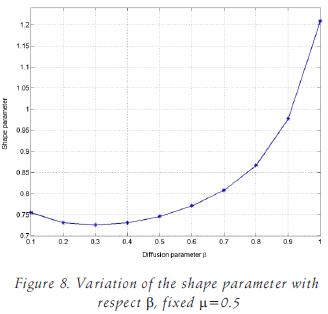
We note that in this numerical experiment, we hold fixed the parameters N, µ and tmax, and that the only variable parameter is β, which in fact characterizes the PDE structure. Therefore, it can be conclude that the determination of the shape parameter is related to the structure of the time dependent advection–diffusion partial differential equation.

 

Conclusions

In this article we investigated the numerical performance of multiquadric collocation methods for a time dependent convection diffusion problem in one dimension. For both implic it and explicit collocation techniques, we found that for moderate Péclet numbers an exponential rate of convergence is at tained. For the explicit technique the time step is restricted by a CFL condition, implying that in order to obtain the same RMS for both schemes, the time step for the explicit method should be one order of magnitude smaller.

We numerically found, that as we increase the Péclet number, for both methods, the slopes of the straight lines in semilog scale which corresponds to the exponential convergence rate are reduced. These results were obtained for h–refinement techniques. We also shown, that exponential rate of convergence is also sat is fied for a c–refinement scheme. More over, we also numerically found that the optimal value of the shape parameter c, de creases monotonically as the Péclet number is increased. This result is a first step towards to determine in an easier way the range of acceptable values of c for which spectral convergence can be at tained. We stress that within the region where the solution presents a sharp gradient, an h–local refinement was used in order to reduce numerical oscillations. This suggest that in order to handle strongly convective dominated problems by means of multiquadric collocation methods, both a an h–c refinement and a domain decomposi tion methods should be used. Recent results in this last direction are in progress and will be published elsewhere.

 

Acknowledgments

The first author would like to thank CONACyT for supporting this work under grant 145052.

 

References

Behrens J., Iske A. Grid–Free Adaptive Semi–Lagran gian Advection Using Radial Basis Functions. Computers and Mathematics with Applications, 43(3–5):319–327. 2002.        [ Links ]

Boztosun I., Charafi A. An Analysis of the Linear Advection–Diffusion Equation Using Mesh–Free and Mesh–Dependent Methods. Engineering Analysis with Boundary Elements, 26(10):889–895. 2002.        [ Links ]

Carlson R.E., Foley T.A. The Parameter in Multiquadric Interpolation. Computers and Mathematics with Applications, 21(9):29–42. 1991.        [ Links ]

Cheng A.H. Golberg M.A., Kansa E.J., Zammito G. Exponential convergence and h–c Multiquadric Collocation Method for Partial Differential Equations. Numerical Methods for Partial Differential Equations , 19(5):571–594. 2003.        [ Links ]

Driscoll T.A., Heryudono A.R.H. Adaptive Residual Subsampling Methods for Radial Basis Function Interpolation and Collocation Problems. Submited to Computers and Mathematics with Applications. 2006.        [ Links ]

Fornberg B., Wright G. Stable Computation of Multiquadric Interpolants for all Values of the Shape Parameter. Computers and Mathematics with Applications, 48(5–6): 853–867. 2004.        [ Links ]

Kansa E.J. Multiquadrics—a Scattered Data Approximation Scheme with Applications to Computational Fluid–Dynamics. II. Solutions to Parabolic, Hyperbolic and Elliptic Partial Differential Equations. Computers and Mathematics with Applications, 19(8–9): 147–161.1990.        [ Links ]

Larsson E., Fornberg B. Theoretical and Computational Aspects of Multivariate Interpolation with Increasing Flat Radial Basis Functions. Computers and Mathematics With Applications, 49(1): 103–130. 2005.        [ Links ]

Li Jichun, Chen C.S. Some Observations on Unsymmetric Radial Basis Function Collocation Methods for Convection–Diffusion Problems. International Journal for Numerical Methods in Engineering, 57(8):1085–1094. 2003.        [ Links ]

Madych W.R., Nelson S.A. Multivariate Interpolation and Conditionally Positive Definite Functions. Mathematics of Computation, 54(189): 211–230. 1990.        [ Links ]

Madych W.R. Miscellaneous Error Bounds for Multiquadric and Related Interpolators. Computers and Mathematics with Applications, 24(12):121–138. 1992.        [ Links ]

Muñoz–Gómez J.A., González–Casanova P., Rodríguez–Gómez G. Adaptive Node Refinement Collocation Method for Partial Differential Equations. IEEE Computer Society: Seventh Mexican International Conference on Computer Science, San Luis Potosi, México, septiembre, pp. 70–77. 2006.        [ Links ]

Rippa S. An Algorithm for Selecting a Good Value for the Parameter c in Radial Basis Function Interpolation. Advances in Computational Mathematics, 11(2–3):193–210. 1999.        [ Links ]

Sarra Scott A. Adaptive Radial Basis Function Methods for Time Dependent Partial Differential Equations. Applied Numerical Mathematics, 54(1):79–94. 2005.        [ Links ]

Schaback Robert Error Estimates and Condition Numbers for Radial Basis Function Interpolation. Advances in Computational Mathematics, 3(3):251–264. 1995.        [ Links ]

Zerroukat M., Djidjeli K., Charafi A. Explicit and Implicit Meshless Methods for Linear Advection–Diffusion–Type Partial Differential Equations. International Journal for Numerical Methods in Engineering, 48(1):19–35. 2000.        [ Links ]

 

About the authors

José Antonio Muñoz–Gómez. He has a PhD degree in Computer Science from National Institute of Astrophysics, Optics and Electronics (INAOE). He is member of the "Sistema Nacional de Investigadores", level candidate. He currently works at the engineering department in University of Guadalajara, campus Autlan. His current research interests include numerical solution of partial differential equations, domain decomposition methods and high performance computing.

Pedro González–Casanova. Is a Researcher at Universidad Nacional Autonoma de México (UNAM) at DGSCA. He has an Under graduate Degree in Physics form Universidad Nacional Autonoma de Mexico and a PhD in Mathematics from Oxford University, GB, where he was research fellow. He is currently area Coordinator of the Mathematical Modeling and Scientific Computation field of the PhD programme in Mathematics at UNAM. He is a member of the "Sistema Nacional de Investigadores", level, II.

Gustavo Rodríguez–Gómez. Received the Bachelor degree and Master degree in Mathematics from the National Autonomous University of Mexico (UNAM). He has a PhD degree in Computational Sciences from the National Institute of Astrophysics, Optics and Electronics (INAOE). His current research interests include scientific computing and the numerical solution of partial differential equations and ordinary differential equations with radial basis functions, multirate methods also called subcycling methods.