Estudios e investigaciones recientes

 

Single and multi–objective optimization of path placement for redundant robotic manipulators

 

Optimización mono–objetivo y multi–objetivo del emplazamiento de trayectorias de robots manipuladores redundantes

 

J.A. Pamanes–García¹, E. Cuan–Durón¹ and S. Zeghloul²

 

¹ Instituto Tecnológico de la Laguna, Dept. of Electric and Electronic Engineering, Torreón, Coahuila, México E–mails: apamanes@itlalaguna.edu.mx, kcuan@itlalaguna.edu.mx and

² Université de Poitiers–Faculté des Sciences, Laboratoire de Mécanique des Solides, CEDEX – France E–mail: Said.Zeghloul@lms.univ-poitiers.fr

 

Recibido: febrero de 2007
Aceptado: octubre de 2007

 

Abstract

General formulations are presented in this paper to determine the best position and orientation of a desired path to be followed by a redundant manipulator. Two classes of problem are considered. In the first, a single manipulator's index of kinematic performance associated to one path point must be improved as much as possible. In the second case distinct indices of kinematic performance, corresponding to different points of the path, are to be optimized. Constraints are taken into account in order to guarantee the accessibility to the whole de sired task. Several case studies are presented to illustrate the effectiveness of the method for planar and spatial manipulators.

Keywords: Optimization, redundant manipulators, path placement, motion planning, kinematic performances.

 

Resumen

En este artículo se presentan formulaciones generales para determinar la mejor posición y orientación de una ruta que se desea que recorra el órgano terminal de un manipulador redundante. Se consideran dos clases de problemas. En el primer caso un índice de desempeño cinemático, asociado a un solo punto de la trayectoria, debe mejorarse tanto como sea posible. En el segundo caso se optimizan distintos índices de desempeño cinemático, correspondientes a diferentes puntos de la ruta deseada. Se consideran restricciones para garantizar la accesibilidad a toda la ruta deseada. Para ilustrar la efectividad del método se presentan varios casos de estudio de manipuladores planares y espaciales.

Descriptores: Optimización, manipuladores redundantes, colocación de trayectorias, planificación de movimientos, desempeño cinemático.

 

I. Introduction

A robot manipulator is kinematically redundant if it has more de gree–of–freedom (dof) than the minimum required for the accomplishment of its tasks.

The redundancy increases the ability of the robot to avoid collisions as well as singular or degenerated configurations when a task is carried out. However, this class of manipulators requires more complex schemes for motion planning compared with non redundant manipulators. Indeed, a redundant manipulator should move in such a way that the end–effector achieves a desired main task and the rest of the arm simultaneously accomplishes a secondary task. The secondary task may be defined as internal motions to optimize manipulator's performances, or to avoid collisions. The kinematic performances can be measured in terms of criteria chosen by the user, like the manipulability (Yoshikawa , 1985) or the condition number (Angeles et al., 1992) of the Jacobian matrix, which are interesting in certain applications.

The redundancy of manipulators has been solved in the literature by optimizing locally (Yoshikawa et al., 1989), (Chiu, 1988) or globally (Nenchev, 1996), (Nakamura et al., 1987), (Pamanes et al., 1999) the kinematic or dynamic performances. In such works it is assumed that the path placement is specified with respect to the robot's frame. Therefore, the performances of the manipulator obtained by applying these methods are relative to the assumed path location. Nevertheless, in some applications, the user could find a suitable path location to improve as much as possible the robot's performances. An automatic turning table or a collaborative manipulator can be used as positioner devices in the robotic workstation to judiciously place the task to the main robot.

The subject of the optimal relative robot/path placement has been studied in the literature mainly for non–redundant manipulators (Zhou et al., 1997), (Nelson et al., 1987), (Fardanesh et al., 1988), (Pamanes, 1989), (Pamanes et al., 1991), (Reynier et al., 1992), (Abdel–Malek, 2000). To the author's knowledge, only J.S. Hemmerle and F.B. Prinz (Hemerle et al., 1991) considered the problem of the optimal path placement for redundant manipulators; in this study, it is assumed that the task is held by a collaborative manipulator (left hand) moving simultaneously with the main manipulator (right hand) which drives the tool. Two criteria of optimization were simultaneously considered: the joint variables were moved away from their limit values as much as possible and the joint displacements were minimized. In that method, however, constraints were not taken into account to assure continuous joint trajectories. On the other hand, the case was not studied in which the task doesn't move simultaneously with the main manipulator; besides, the optimization of kinematic performances on specific zones of the path was neither investigated. The resolution of both problems becomes interesting in industrial applications.

Two cases of optimal path placement are studied in this paper for redundant manipulators. In the former (single–objective problem) we formulate a process to compute the path placement which allows to optimize one index of kinematic performance of the manipulator on only one point of the desired path. In the second case (multi–objective problem) we compute the path placement such that distinct indices of kinematic performance are optimized on different zones of the path. Constraints are taken into account in order to avoid both exceed the joint limits and discontinuous joint trajectories.

In the next section some concepts of robot kinematics are evoked which are later applied in our formulations. A solution is presented in the third section for the single–objective problem and then, in the fourth part of the paper, the multi–objective problem is studied. The generalization of our formulations to solve the case of global optimization is observed in the fifth section. Some case studies are discussed to illustrate the effectiveness of the methods for both planar and spatial manipulators. The concluding remarks are finally presented.

 

II. Preliminaries

The kinematic function of a robot manipulator is defined as:

x = f(q)                        (1)

where x is the m–dimensional vector of operational coordinates describing the situation of the end–effector in the Cartesian space; q is the n–dimensional vector of joint variables defining the instantaneous configuration of the manipulator; f is an m–dimensional function (n > m).

The inverse kinematic function of a manipulator, if it exists, is given by

q = f ^–1(x)                        (2)

The direct velocity function of a robot manipulator is obtained by differentiation of equation 1:

where the dot denotes differentiation with respect to time and is the Jacobian matrix of the manipulator. When the number n of joint variables q_i of a manipulator is equal to the number m of operational coordinates x_j of the end effector, then the manipulator is called non redundant. On the other hand, when n > m the manipulator is termed redundant. In this case the inverse kinematic function of equation (2) has an infinite number of solutions.

The inverse velocity function of a manipulator is obtained from equation 3 as

If J (q) is singular or n > m then the inverse J ^–1(q) does not exists and the linear system of equation (3) cannot be solved by using equation (4). In such a case the inverse velocity function may be expressed as

where

J⁺ is the pseudo–inverse of J (in order to simplify the terms in this paper J(q) will be equivalent to J).

z is an arbitrary vector .

I is the identity matrix of dimension n'n.

In equation (5), is the least–norm solution of equation (3), i.e., it provides a vector with minimum Euclidean norm satisfying this Equation. On the other hand, (I–J⁺ J) z represents the projection of z on the null–space of J; this part is called the homogeneous solution of equation (3); it is referred to as the self–motion of the manipulator and does not cause any end–effector motion. In order to use the self–motion to improve configurations, the vector z is chosen as

where

h(q) is the gradient of an index of performance h(q) to be optimized.

k is a scaling factor of h(q). It is taken to be positive if h(q) must be maximized and negative if h(q) is to be minimized.

Several criteria of kinematic performances for manipulators have been proposed in the literature, which can be considered for the index h(q) in equation (6). Each of such indices evaluates different kinematic features of a manipulator, which may be interesting depending on the nature of the task to be carried out. A succinct survey of two indices of performance is presented below. Such indices, the manipulability and the condition number of the jacobian matrix, will be applied as criteria of optimization to solve the path placement problems in section VI.

The manipulability index, introduced by Yoshikawa (1985), is defined as

The manipulability is a measure of the ability to arbitrarily change the position or orientation of the end effector.

Thus, its maximization would be appreciated in task zones where relatively large deviations in the prescribed motion of the end–effector are likely.

The condition number of the Jacobian matrix is another interesting index applied to evaluate the performances of robotic manipulators (Angeles et al., 1992). Such index can be computed as:

where µ_max is the largest singular value of J and µ_min is the smallest singular value of J.

The minimum condition number of a manipulator minimizes the error propagation from input joint velocities to output end–effector velocities. Thus, it can be used as a local measure of accuracy of the manipulator's motions.

 

III. Optimal path placement for single–objective optimization

A. Statement of the problem

The task of a n–dof manipulator is specified by a set of n_t m–dimensional vectors of operational coordinates of the end–effector in an orthonormal frame Σ_t The manipulator considered is assumed as being redundant (n>m). The n_t vectors correspond to a sample of points p_i (i = 1, 2, ..., n_t) of the desired path in the task space. The operational coordinates are the desired positions and orientations of the frame Σ_n+1 attached to the end–effector, as showed in figure 1.

A suitable index of performance is then assigned by the user to one arbitrary path point, say p_k, k {1,..., n_t}, which must be maximized by the corresponding manipulator's configuration when the task will be accomplished. A law of motion is also given which refers to the time the position of the end effector on the path.

On the other hand, the path placement is specified by variables regarding the position and orientation of the frame Σ_t with respect to the frame Σ₀ fixed to the base of the robot. They are the components of the placement vector defined as

 0 e = [r_tx, r_ty, r_tz, α,β, γ]^T                        (9)

where r_tx, r_ty, r_tz, are the orthogonal components of the vector of position °r_t (Figure 1), and α, β, γ are the Euler angles Z–Y–X defining the orientation of Σ_t with respect to the frame Σ₀ .

It is desired to obtain the components of the placement vector ⁰e of the path, so that the index of manipulator's kinematic performance associated to the sample point p_k is optimized when the task is accomplished.

 

B. Process of solution

The single–objective problem is equivalent to a constrained non–linear programming problem. The objective function is defined as the index of performance h_k(q_k ) assigned to the path point p_k. The number of independent variables will be generally 6+n: the 6 components of the placement vector ⁰e of the path and, because of the manipulator's redundancy, the n joint variables of the configuration q_k which allow to satisfy the desired situation of the end–effector at the path point p_k.

To solve the problem, we propose an optimization process in three phases: phase I in which the optimal placement vector must be found; phase II addressed to compute the optimal configuration on the path point p_k for each proposed placement to be evaluated; and phase III committed to complete the manipulator's joint trajectories for the whole desired path by using the optimal path placement obtained in phase I. Notice that phase II allows to evaluate the objective function of phase I. Such a function in phase I can be defined as

f = h_k (q_k)                                                   (10)

The general procedure to solve the single–objective problem is schematized in the flow chart of figure 2. Details on the three phases concerned are given below.

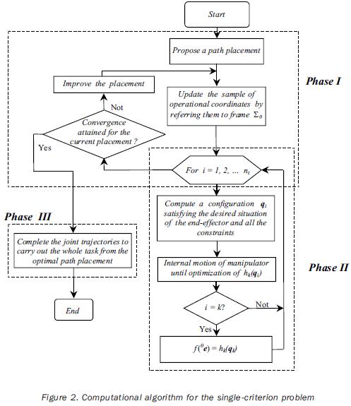
Phase I

Before obtain the configurations at each path point, the operational coordinates must be referred to frame Σ₀. Therefore, when a new placement is proposed in the optimization process, the operational coordinates have to be first updated in phase I by applying the following transformation:

 ⁰ T _l = ⁰ T_{t ^t}T_l                                                   (11)

In this equation:

^tT_l is the homogeneous matrix establishing the desired position and orientation of the end effector on the path point p_i referred to frame Σ_t

⁰T_t is the homogeneous matrix for the position and orientation of frame Σ_t referred to frame Σ₀.

⁰ T_i is the homogeneous matrix defining the position and orientation of the end effector on the path point p_i with respect to frame Σ₀

When the given operational coordinates have been updated, then the objective function must be evaluated in phase II for the current placement; after the process returns to phase I in order to check for the convergence of the method. If the convergence is attained then the procedure goes to phase III; otherwise, the placement must be improved by applying a suitable strategy.

 

Phase II

After updating of the operational coordinates for a path placement proposed in phase I, the redundancy must be solved to find the configurations q_i (i=1, 2, .... n_t) for all the path points. To do that, we assume as secondary task on point p_i the optimization of the same index of performance considered on p_k; i.e., for one path point the manipulator has to achieve the corresponding operational coordinates and also optimize h_k(q_i). To find such configurations the following process is carried out:

1. Find a configuration q_i at each path point in such a way that Equation (1) is satisfied. This configuration is obtained by minimization of the following function:

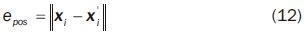
where x_l is the vector defining the desired situation of the end–effector at point p_i, and x_i' is a vector of operational coordinates corresponding to a configuration q_l' proposed when minimizing of equation (12). The symbol denotes the Euclidean norm. If the task is feasible then equation x _l = x_l' will be satisfied when the norm of equation (12) is minimized. The numeric minimization is carried out by applying a method of constrained non–linear optimization. The independent variables are the joint variables of q_l'. The constraints to be considered are presented in the next sub–section.

2. When a configuration qi at one path point has been found, satisfying both equation (1) and all the constraints, then compute J, J⁺and, h(q) and optimize for such a configuration the index h(q) by successively obtaining of the homogeneous solution of equation (3). At each iteration of this process, when a vector q_i of the homogeneous solution is obtained corresponding to a certain configuration q_i , an improved configuration q_i* may be computed by

where Δ is a sufficiently small time interval. Note that, because is a homogeneous solution, the improved configuration q_i* will also preserve equation (1). The initial configuration of the optimization process has been determined in step i.

3. For one path–point the optimization of a configuration is stopped when becomes zero.

 

Phase III

When computing the optimal path placement only a significant sample of path points is considered in order to reduce the time of computation engaged in the optimization process. Nevertheless, the desired trajectory is a continuous curve which must be approximated by a sufficiently large number of supplementary points of the path. So, to synthesize continuous joint trajectories for the whole task, when the optimal placement has been found the redundancy must be solved for supplementary path points. This process is the same used to solve the redundancy in phase II by optimizing the desired index of performance h_k(q). The number of supplementary points is proposed by the user in such a way that a conventional precision be satisfied. Continuous joint trajectories will be obtained as a result of this process because the index to be optimized is the same for all the considered points.

C. Constraints of the problem

The optimization processes to obtain the path placement and to solve the redundancy must be constrained in order to obtain realistic solutions. The following constraints are taken into account:

1. Explicit constraints in phase I

Explicit constraints are imposed in phase I on the placement vector so that solutions are obtained only into the available physical space for the task placement. Such space may be imposed by a positioner device. The following constraints on the components of the placement vector are considered:

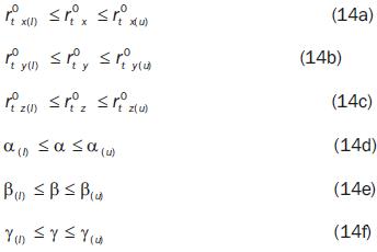
In expressions (14), the indexes l and u denote, respectively, lower and upper bounds of the independent variables.

2. Implicit constraints in phase I for access to the task

Implicit constraints are also considered in order to guarantee the efficacy of placements proposed in the optimization process. To assure the accessibility to all the sample points on the path the following constraint is introduced:

where t _l is the reach vector demanded to the manipulator at point p_i; the symbol denotes Euclidean norm. t_u is the norm of the maximum reach which the manipulator can provide. Such norm depends on the geometric parameters of the manipulator.

3. Explicit constraints in phase II for joint limits avoidance

An elemental condition for any feasible configuration consists in preserving the joint variables into the admissible domain of configurations. So, any configuration used for the task should verify the following conditions:

where:

q_ij is the i–th joint variable of the q_j manipulator's configuration corresponding to the j–th task point.

q^(l)q^(u) are the lower and upper limits, respectively, of the i–th joint variable.

4.     Implicit constraints in phase II to guarantee continuous joint trajectories

Implicit constraints are imposed in phase II which allow to assure the feasibility of the whole joint trajectories.

To introduce the considered constraints we recall here de notion of the aspect of a manipulator. One aspect is defined (Borrel et al., 1986) as a continuous subset of the manipulator's joint space composed by configurations which render non–zero all the m–order minors of the jacobian matrix, except those minors being zero everywhere in the joint space.

Thus, the aspects of a manipulator are subsets of the joint space separated by hypersurfaces whose equations are determined by the m–order minors of the jacobian matrix equalized to zero.

On the other hand, it is known that for non–cuspidal manipulators (Burdicket al., 1995), (Wenger, 1997), the continuity of joint trajectories corresponding to a given task can be guaranteed if the manipulator is constrained to use configurations remaining in only one aspect of its joint space.

Consequently, to guarantee continuous joint trajectories the following conditions must be imposed to manipulator's configurations which will be used to accomplish a desired path:

 ε_kj δ_kj (q) > 0                  (17)

where

δ_kj (q) is the left hand function of the equation defining the j–th hypersurface (j = 1, 2,..., n_hk ) which borders the aspect A_k in the joint space; . n_hk is the number of such hypersurfaces. n_A is the number of the robot's aspects. Only one aspect will be chosen containing all the configurations which allow to achieve the desired task.

ε_kj is a constant (+1 or –1) depending on the hypersurface and the considered aspect A_k.

In section VI we will identify the implicit constraints (17) for two manipulators.

 

VI. Optimal path placement for multi–objective optimization

A. Statement of the problem

The task of a n–dof manipulator is specified by a set of n_t m–dimensional vectors of operational coordinates of the end–effector (n>m) in an orthonormal frame Σ _t. Such operational coordinates give the desired positions and orientations to be followed by a frame Σ_n+1 attached to the end–effector, as showed in figure 1. In that figure a sample of points p_i (i = 1, 2, ..., n_t ) is illustrated corresponding to the desired path in the task space. Suitable indexes of performance are then assigned by the user to several path points p_i. Thus, we want to compute the path placement vector ⁰e, so that all the indexes associated to the sample points be optimized while the task is being accomplished. A law of motion is also specified which refers to the time and position of the end–effector on the path.

B. Process of solution

The multi–objective problem is also a constrained non–linear programming problem. The objective function should consistently characterize a set of dissimilar indexes of performance to be optimized. Thus, it is required that the indexes be first normalized to eliminate scaling and unity differences; then they can be included in a coherent objective function.

As in the single–objective problem, the independent variables will be the 6 components of the path placement vector ⁰e and, because of the manipulator's redundancy, the joint variables of configurations q_i which allow to satisfy the desired situation of the end–effector on the path points p_i. To solve the multi–objective problem we propose an optimization process having also three phases. In phase I the optimal placement will be searched; phase II is addressed to compute the optimal configurations at the n_t path points for each placement to be evaluated; phase III is finally committed to synthesize the manipulator's joint trajectories for the whole desired path by using the optimal path placement obtained in phase I. Note that phase II allows to evaluate the objective function of phase I. Such a function is defined below. The procedure presented here to solve the multiobjective problem is illustrated in the flow chart of Figure 3. Details of the procedure are discussed in the next paragraphs.

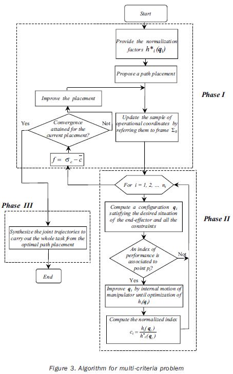
Phase I

The path placement must be searched in this phase. For each placement proposed here we have to update the operational coordinates; then an evaluation of the placement can be accomplished in the process of optimization.

The transformation of such coordinates is carried out by applying equation (11); then the redundancy will be solved in phase II, and the objective function will be computed based on normalized indexes of performance. After that the process returns to Phase I in order to check for the convergence of the method. If the convergence is attained then the procedure goes to Phase III; otherwise, the placement must be improved by applying a suitable strategy. The objective function for the multi–objective problem as well as the normalized indexes, are defined below.

A normalized index of performance associated to the sample point p_i is obtained as:

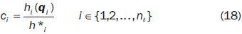
The normalization factor h_i* in equation (18) is the maximum value of the index of performance at the point p_i that can be obtained by the manipulator when only such index is optimized, and the accessibility to all the path points is satisfied. In fact, the normalization factor h_i* is the optimal value obtained for the index h_i (q_i) in the single–objective problem. Thus, to obtain the normalization factors we have to solve as much single–objective problems as sample–configurations are to be optimized. It must be observed that a sample–point could hold or not an index of performance associated to be optimized; thus, the number of indexes to be optimized can be lower or equal than n_t.

The main idea to define the objective function is that the value of such function, corresponding to a path location, must be equivalent to a typical value of the set of normalized indices to be optimized. Such typical value can be defined as:

where and are, respectively, the mean and the standard deviation of the set of normalized indexes associated to the sample points. Hence, the value of c obtained by equation (19) corresponds to a typically small value of the set of normalized indexes of the sample.

If we assume that the all the indexes of performance considered in the problem are to be maximized, then the global maximization of the set of n_t indexes would be obtained by maximization of c. Nevertheless, algorithms in usual software for optimization are generally intended to minimize the objective function. Thus, to solve the optimization problem by minimization, the objective function could be defined as – c; therefore, such a function can be finally written as:

Phase II

The n_t optimal configurations satisfying the desired task and constraints, which are used to compute the normalized indexes, must be found in phase II. The algorithm to compute such configurations is the same used in single–objective problem; this one has been described in section III.

Phase III

The continuous joint trajectories for the whole task must be finally synthesized in Phase III for the optimal path placement. To do that, the redundancy has to be solved for supplementary path points in such a way that the optimal configurations of points p_i obtained in phase II are preserved.

In the multi–objective problem however, because of generally different indexes of performance are associated to adjacent sample path points, say p_i and p_i+1 , we cannot use a single index to solve the redundancy by using the homogeneous solution for intermediate path points. In fact, if the homogeneous solution is applied on intermediate points to optimize the index associated to p_i, then the joint trajectories becomes discontinuous on p_i+1 and vice versa.

To solve the redundancy and synthesize the continuous joint trajectories connecting adjacent sample path points, a judicious strategy must be used. We propose a suitable secondary task to be accomplished, which is specified in the joint space as a continuous trajectory between configurations associated to adjacent sample path points. This secondary trajectory is such that the determinant of J J^T smoothly evolves from its value on point pi to the value on point p_i+1. Consequently, because all the configurations so obtained belong to only one aspect, the continuity of joint trajectories will be assured. Thus, to accomplish both the main and the secondary tasks, we propose to solve the redundancy by minimizing the following objective function at each intermediate point p_j between two successive sample points p_i and p_i+1:

where n_int is the number of intermediate points to be considered between two sample points. This number is chosen by the user so that a conventional precision be satisfied. The error of position of the end–effector, e_{pos j}, in equation (21), is defined like in equation (12) for intermediate points.

On the other hand, we define J*_J = J_i J_i^T, where J_i is the Jacobian matrix of the manipulator on the intermediate point p_j. Then the error of the determinant of J*_j in equation (21) is defined as

det J*_J is the desired value of the determinant of J* for the configuration at point p_J . Its value is assigned by a cycloidal law [Equation (23)] which is defined for the current segment of the path between two successive sample points. Such cycloidal law must smoothly change the determinant of J* from its value corresponding to the configuration at point p_i, to that one at p_i+1.

det J_i' is the value of the determinant of J* for the current configuration in minimization of equation 21.

The desired behavior of the determinant of J* in the segment between sample points p_i and p_i+1 is described by the following cycloidal law:

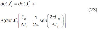
The variables concerned in equation (23) are defined as follows:

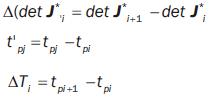
where t_pi, t_pj are the values of the time elapsed when the end–effector arrives at points p_i (sample) and p_j (intermediate), respectively.

C. Constraints of the problem

As considered for the single–objective problem, to obtain realistic solutions in solving the multi–objective problem, explicit and implicit constraints should also be taken into account. Such constraints are identical to those considered in Section III C. They were examined in that section.

 

V. Path placement for global optimization

The path placement problem was studied in section III for the optimization of manipulator's performance on a certain point of the path by taking into account a single kinematic criterion. Nevertheless, in some tasks the optimization of such criterion can be preferred not only on a particular point but on every one of points in the path; i.e. a global optimization of manipulator's performances is desired when the task is carried out. Note that such problem can be considered as a particular case of the multi–objective problem examined in the previous section. In fact, in the formulation for multi–objective optimization we can assign the same criterion of performance to all the sample points in order to attain the global optimization. However, it must be pointed out that the homogenization of the corresponding indices is not required in the process of solution; then equation (18) takes the form c_i = h_i (q_i).

Furthermore, after optimizing the set of indexes on the sample points, the continuous trajectories of joint variables for the whole path can be synthesized by applying only the Phase III of the process for the single–objective problem. Consequently, the minimization of function (21) is not necessary for global optimization.

 

VI. Case studies

Several case studies are presented in this section in which single and multi–objective problems of optimal path placement are solved; we consider planar and spatial paths for each kind of problem. The planar task must be accomplished by a 3R manipulator, and the spatial task should be achieved by a 4R manipulator. In the following sub–section, the geometric parameters of both manipulators will be specified and the implicit constraints of the problems to hold configurations in an aspect will be identified. Then, in succeeding subsections the problems will be solved.

A. Manipulators for the case studies

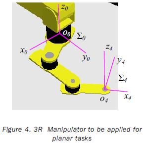
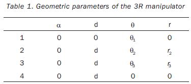
1. The 3R manipulator

The considered planar manipulator is shown in Figure 4, and its geometric parameters are presented in table 1. These parameters are defined by using the modified Denavit–Hartenberg method (Khalil et al., 1986). A frame Σ₄ is attached at the tip of the third link in order to use its origin to specify the linear velocity of the end–effector. The manipulator's joint variables are θ₁, θ₂ and θ₃, and its limit values are θ_i^(l) =–150° and θ_i^(u) =150°, for i = 1, 2, 3 .

By considering the velocity vector of O₄ referred to the frame Σ₀ as , the jacobian matrix of the manipulator is:

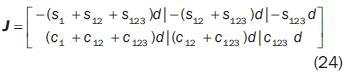
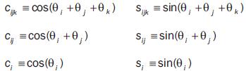
In this matrix and hereafter we use the following compact notation:

The 2–order minors of the jacobian matrix are expressed as:

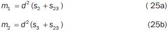
The conditions of configurations which render zero the above minors provide the following equations of the surfaces dividing the joint space in aspects:

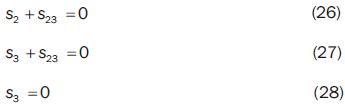
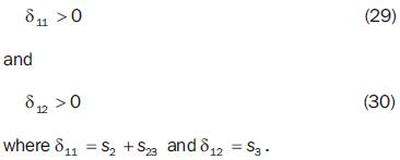
Thus, six aspects can be identified (n_A=6) for the 3R manipulator, as showed in figure 5. We chose the aspect A₁ for the achievement of the task; consequently for (17) we have k=1. Then we observe that the aspect A₁ is surrounded by the surfaces specified by equations (26) and (28); therefore we have n_hk =2 and ε₁₁=1, ε₁₂=1 for inequality (17).

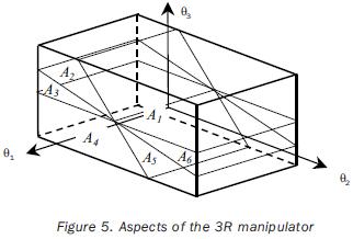
The implicit constraints on θ₂ and θ₃ to hold configurations in the aspect A₁ are then expressed as

 

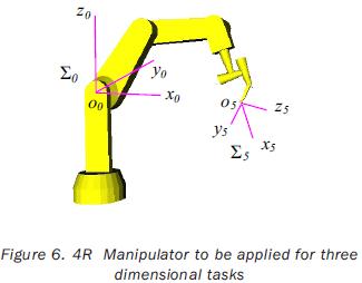
2. The 4R manipulator

The manipulator is shown in figure 6 and its geometric parameters are presented in table 2. The joint variables are θ₁, θ₂, θ₃ and θ₄, and its limits values are θ_i^(l) = –150° and θ_i^(u) = 150°, for i = 1, 2, 3, 4. To specify the linear velocity of the end effector we use the point O₅ of the frame Σ ₅ which is attached at the tip of the fourth link.

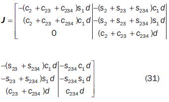
By considering the velocity vector of O₅ referred to the frame Σ₀ as , the jacobian matrix of the 4R manipulator is:

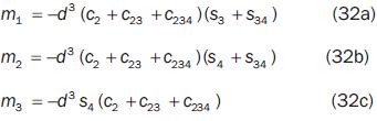
The 3–order minors of the jacobian matrix which are non zero everywhere in the joint space are:

The conditions of configurations which render zero the above minors provide the following equations of the surfaces dividing the joint space in aspects:

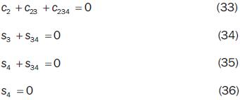
Thus, twelve aspects can be identified (n_A=12) for the 4R manipulator. We chose the aspect A₁ for the achievement of the task; consequently, for inequality (17) we have k=1. Then we observe that the aspect A₁ is bounded by the surfaces of equations (33), (34) and (36); therefore for inequality (17) we have n_hk=3 and ε₁₁=1, ε₁₂=1, ε₁₃=1. Thus, the implicit constraints on configurations to hold configurations in the aspect A1 are:

 δ₁₁ > 0                  (37)

 δ₁₂ > 0                  (38)

 δ₁₃ > 0                  (39)

where

 δ₁₁ = c₂ + c₂₃ + c₂₃₄ + δ₁₂ = s ₃ + s ₃₄

and

 δ₁₃ = s₄

 

B. Single–objective problems

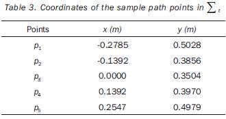
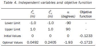
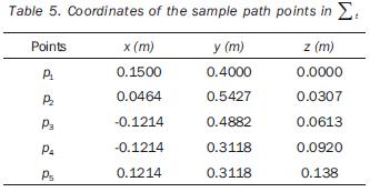
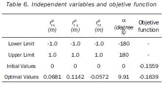
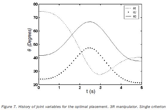
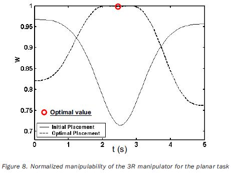
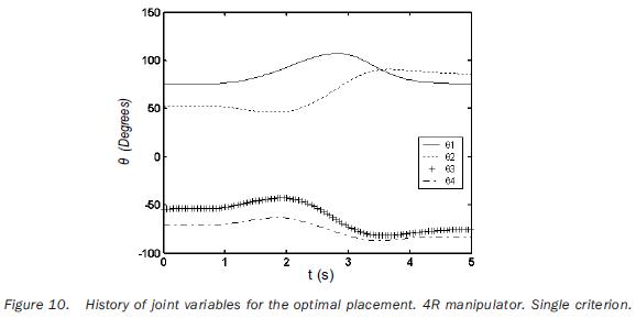
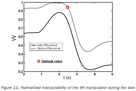
The tip of the 3R manipulator should complete a parabolic path; whereas in the case of the 4R manipulator, the tool has to describe a helicoidal path. The tasks of both robots are to be accomplished by applying cycloidal laws of motion to the end–effector during 5 seconds. The Cartesian coordinates of the sample–points are referred to the frame Σ_t; they are given in tables 3 and 5. (table 3, 4 and 5). In the two cases the path placements must be determined in such a way that the manipulability index is maximized on the point p₃ (when t=2.5 s). The independent variables of the planar problem are r_t°_x, r_t°_y, and α (rotation about the axis z₀ ); in the case of the 3D path, the additional variable r_t°_z must be included. The initial values for such variables, as well as the obtained optimal values are given in tables 4 and 6. In the same tables the initial and a the optimal values of the objective functions are presented. The joint trajectories corresponding to the optimal placement are observed in figures 7 and 10 (Figures 7, 8, 9 and 10). The behaviors of the normalized manipulability are compared in figures 8 and 11. Sequences of configurations of the robots during the accomplishment of the tasks are presented in figures 9 and 12 for the initial and the optimal placements.

B1. Parabolic path

B2. Helicoidal paht

 

C. Multi-objetive problems

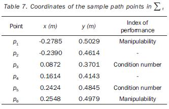
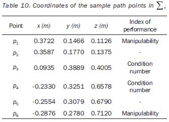
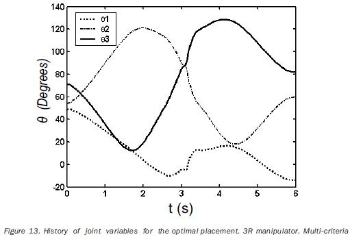
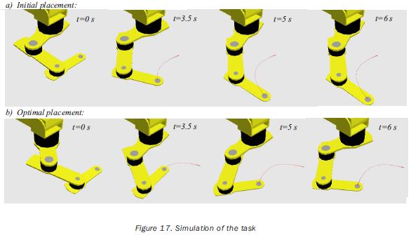
In the case of the planar task the extremity of the 3R manipulator should complete a parabolic path; for the 3D task the 4R manipulator's tool has to describe a helicoidal path. In both cases the motion of the end–effector follows a cycloidal law. The periods of the tasks are 6 and 5 seconds for the 3R and 4R manipulators, respectively. The Cartesian coordinates of the sample–points are referred to frame Σ_t, and different indexes of performance are associated to some points, as indicated in tables 7 and 10. (table 7, 8, 9 and 10). In the problems we want to determine the path placement which allows to optimize the value of the specified indexes by the related manipulator's configuration when the task is carried out.

1. Parabolic path

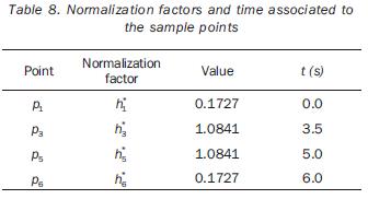
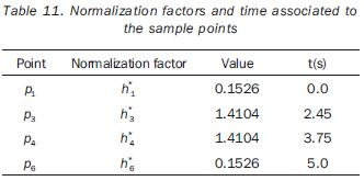
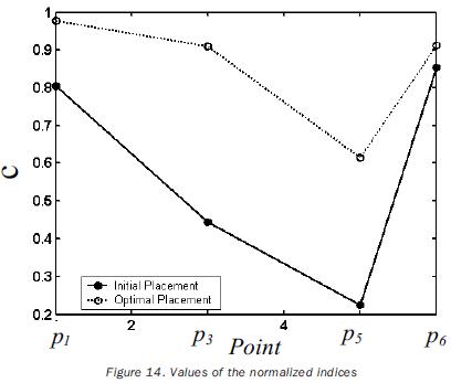
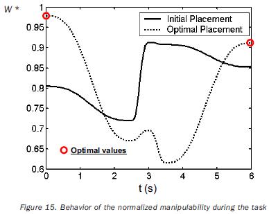
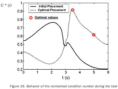
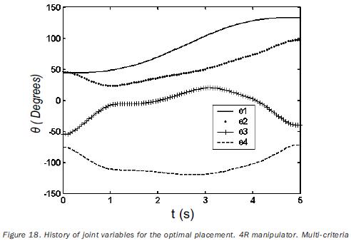
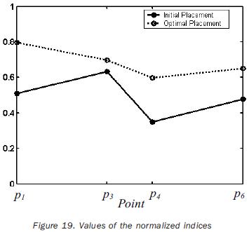
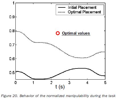
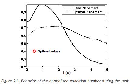
The normalization factors used in equation (18) are previously computed by solving the single–objective problem for points having a related index of performance. The obtained values of such factors are listed in tables 8 and 11. The independent variables of the planar problem are r_t°_x, r_t°_y and a (rotation about the axis z₀); in the case of the 3D path, the additional variable r_t°_y must be included. The initial values for such variables, as well as the obtained optimal values are given in tables 9 and 12. In the same tables the initial and optimal values of the objective functions are presented. The joint trajectories corresponding to the optimal placement are observed in figures 13 and 18. The progress attained of the normalized indices associated to the sample points can be appreciated in figures 14 and 19. The behaviors of the manipulability and the condition number (both normalized) during the task are shown in figures 15, 16, 20 and 21. Sequences of configurations of the robots describing the desired paths are presented in figures 17 and 22 for the initial and the optimal placements.

 

Conclusion

General formulations were presented in this paper to determine the best position and orientation of a path to be followed by a redundant robotic manipulator. Depending on the requirements of the user, the quality of a placement can be measured by using either a single criterion or multiple criteria of manipulator's performance. Consequently, the proposed formulations are addressed to solve both single and multi–objective optimization problems. In the single–objective problem, one index of performance associated to a specific path–point is defined as the function to be optimized. On the other hand, in the multi–objective problem such a function is equivalent to a characteristic index which represents the set of normalized indexes to be optimized. The proposed formulations take into account constraints regarding the accessibility to the manipulator's task. Indeed, we introduce constraints in order to: a) demarcate an available physical space to locate the task; b) avoid transgression of joint limits during the accomplishment of the task; c) generate continuous joint trajectories on the whole task.

The case studies examined here showed that significant improvements of the manipulator's performance can be obtained by applying our approach. In such cases all the constraints were satisfied and consequently the accessibility to the complete tasks was assured. However, in the hypothetical case in which a satisfactory solution could not be found by trying with a first manipulator's aspect, then further attempts could be accomplished by using other manipulator's aspects to satisfy the accessibility conditions and improve the manipulator's performance. On the other hand, the sample points considered in the problems were chosen by using a criterion of symmetry; nevertheless, both the number of points and the position of such points on the path could have an influence on the level of the improvement obtained for the indices of performance. Thus, supplementary studies should be carried out to characterize a suitable criterion to solve both questions. Furthermore, in future works additional constraints will be taken into account to avoid collisions of the manipulator when it works in cluttered environments.

 

Acknowledgments

The subvention for cooperation between researchers of the Instituto Tecnológico de la Laguna of Mexico and the Laboratoire de Mécanique des Solides of France for this work was made possible under the grant M00 M02 ECOS–CONACyT–ANUIES. On the other hand, a part of the present work was supported by the National Council of Science and Technology –CONACyT– of Mexico, (grant 31948–A).

 

References

Abdel–Malek S. and Nenchev D.N. Local torque minimization for redundant manipulators: a correct formulation. Robotica, 14:235–239, 2000.        [ Links ]

Angeles J. and López–Cajún C. Kinematic isotropy and conditioning index of serial robotic manipulators. Int. J. Robotics Research, 11(6):560–571, 1992.        [ Links ]

Aspragathos N.A. and Foussias S. Optimal location of a robot path when considering velocity performance. Robotica, 20:139–147, 2002.        [ Links ]

Borrel B. and Liegois A. A study of multiple manipulator inverse kinematic solution with applications to trajectory planning and workspace determination. IEEE Proc. of the 1986 International Conference on Robotics and Automation, pp. 1180–1185.        [ Links ]

Burdick J.W. A classification of 3R regional manipulator singularities and geometries. Mechanisms and Machine Theory, 30(1): 71–89, 1995.        [ Links ]

Chiu S.L. Task compatibility of manipulators postures. Int J. Robotics Research, 7(5):13–21,1988.        [ Links ]

El Omri J. and Wenger P. How to recognize simply a non–singular posture changing 3–DOF manipulator. Proceedings of the 7^th International Conference on Advanced Robotics, 1995, pp. 215–222.        [ Links ]

Fardanesh B. and Rastegar J. Minimum cycle time location of task in the workspace of a robot arm. IEEE Proc. of the 21st Conference on Decision and Control, 1988, pp. 2280–2283.        [ Links ]

Hemerle J.S. and Prinz F.B. Optimal path place ment for kinematically redundant manipulators. Proceedings of the 1991 IEEE International Conference on Robotics and Automation, 1991, pp. 1234–1243.        [ Links ]

Hsu D., Latombe J.C. and Sorkin S. Placing a robot manipulator amid obstacles for optimized Execution. IEEE Int. Symp. on Assembly and Task Planning, 1999.        [ Links ]

Khalil W. and Kleinfinger J.F. A new geometric notation for open and closed–loop robots. In: Proceedings of the IEEE International Conference on Robotics and Automation, 1986, pp. 1174–1180.        [ Links ]

Klein C.A. and Blaho, B.E. Dexterity measures for the design and control of kinematically redundant manipulators. Int. J. Robotics Research, 6 (2):72–83, 1987.        [ Links ]

Nakamura Y. and Hanafusa H. Optimal redundancy control of robot manipulators. Int. J. Robotics Research, 6(1):32–42, 1987.        [ Links ]

Ma S. and Nenchev D.N. Local torque minimization for redundant manipulators: a correct formulation. Robotica, (14):235–239, 1996.        [ Links ]

Nelson B., Pedersen K. and Donath M. Locating assembly tasks in a manipulator's workspace. IEEE Proc. of the International Conference on Robotics and Automation, 1987, pp. 1367–1372.        [ Links ]

Pamanes G. J. A. A criterion for optimal place ment of robotic manipulators. IFAC Proc. of the 6th Symp. on Information Control Problems in Manufacturing Technology, 1989, pp.183–187.        [ Links ]

Pamanes G.J.A and Zeghloul S. Optimal place ment of robotic manipulators using multiple kinematic criteria. Proceedings of the 1991 IEEE International Conference on Robotics and Automation, 1991, pp. 933–938.        [ Links ]

Pamanes G.J.A., Barrón L.A. and Pinedo C. Constrained optimization in redundancy resolution of robotic manipulators. Proceedings of the 10th World Congress on Theory of Machines and Mechanisms, Oulu, Finland, 1999, pp. 1057–1066.        [ Links ]

Reynier F., Chedmail P. and Wenger P. Optimal positioning of robots: feasibility of continuous trajectories among obstacles. IEEE Int. Conf. on Systems Man. and Cybernetics Proc., 1992.        [ Links ]

Wenger P. Design of cuspidal and noncuspidal manipulators. Proceedings of the IEEE International Conference on Robotics and Automation, 1997, pp 2172–2177.        [ Links ]

Yoshikawa T. Manipulability of robotics mechanisms. Int. J. Robotics Research, 4(2):3–9,1985.        [ Links ]

Yoshikawa T. and Kiriyama S. Four–joint redundant wrist mechanism and its control. Journal of Dynamic System, Measurement, and Control, 111:200–204, 1989.        [ Links ]

Zeghloul S. and Pamanes G.J.A. Multi–criteria placement of robots in constrained environments. Robotica, 11:105–110, 1993.        [ Links ]

Zhou Z.L., Charles C. and Nguyen. Globally optimal trajectory planning for redundant manipulators using state space augmentation method. Journal of Intelligent and Robotic Systems, Vol. 19(1):105–117, 1997.        [ Links ]

 

Semblanza de los autores

J. Alfonso Pamanes–García. Was born in Torreon, Mexico, in 1953. He received the B.S. degree from the La Laguna Institute of Technology in 1978, the M.S. degree in mechanics in 1984 from the National Polytechnic Institute of Mexico, and the Ph.D. degree in mechanics from the Poitiers University, France, in 1992. He is a professor in mechanics of robots at the La Laguna Institute of Technology, Torreon, Mexico. His research interests are in modeling and motion planning of robots. Author of more than 50 scientific papers published in national or international congress and journals. He has been reviewer of the National Council of Science and Technology of Mexico for evaluation of national research projects.

Saïd Zeghloul. Received the M.S. degree in mechanics and the Ph.D. degree in robotics from the University of Poitiers, France, in 1980 and 1983, respectively, and the Doctorat d'Etat es sciences physiques degree in 1991. He is a professor at the Faculte des Sciences of the Poitiers University where he teaches robotics. He is leader of the research group in robotics of the Laboratoire de Mecanique des Solides of Poitiers, where his research interests include mobile robot and manipulator path planing, mechanical hand grasp planing.

Enrique Cuan–Durón. Was born in Torreon, Mexico, in 1960. He received the B.S. degree from the La Laguna Institute of Technology in 1981, the M.S. degree in computer systems in 1985 from the Institute of Technology and Superior Studies of Monterrey. He develops his Ph.D. thesis at the Poitiers University, France, with the support of the La Laguna Institute of Technology, Torreon, Mexico. His main research interests are in motion planning and redundant robots.