Estudios e investigaciones recientes

 

Theoretical model of discontinuities behavior in structural steel

 

Modelo teórico del comportamiento de discontinuidades en acero estructural

 

F. Casanova del Angel¹ and J.C. Arteaga–Arcos²

 

¹SEPI – ESIA ALM– IPN, México
jcarteaga_mx@yahoo.com.mx

²CITEC – IPN, México and
fcasanova@ipn.mx

 

Recibido: junio de 2006
Aceptado: octubre de 2007

 

Abstract

The theoretical development of discontinuities behavior model using the complex variable theory by means of the elliptical coordinate system in order to calculate stress in a microhole in structural steel is discussed. It is shown that discontinuities, observed at micrometric levels, grow in a fractal manner and that when discontinuity has already a hyperbolic shape, with a branch attaining an angle of 60 in relation to the horizontal line, stress value is zero. By means of comparing values of stress intensity factors obtained in the laboratory with those obtained using the theoretical model, it may be asserted that experimental values result from the overall effect of the test on the probe.

Keywords: Micro discontinuities, fractal, structural steel, stress intensity factor, Chevron–type notch.

 

Resumen

Se presenta el desarrollo teórico del modelo de comportamiento de discontinuidades que hace uso de la teoría de variable compleja, mediante el sistema de coordenadas elípticas para el cálculo del esfuerzo en un micro agujero en acero estructural. Se muestra que la forma del crecimiento de las discontinuidades, observadas éstas a niveles micrométricos, es del tipo fractal, y que cuando la discontinuidad ha tomado ya una forma hiperbólica, donde alguna de sus ramas alcanza un ángulo igual a 60 con respecto a la horizontal, el valor del esfuerzo vale cero. Comparando los valores de los factores de intensidad de esfuerzos obtenidos en laboratorio y los obtenidos con el modelo teórico, se puede afirmar que los valores experimentales son el resultado de los efectos globales de la prueba sobre la probeta.

Descriptores: Micro discontinuidades, fractal, acero estructural, factor de intensidad de esfuerzos, muesca tipo Chevron.

 

Introduction

Based on the idea that every structure might crack, this research is the result of observing appearing cracks and their corresponding structural consequences. This allows us to better understand the apparition and behavior of fissures, which phenomenon in structural engineering is very interesting for many researchers.

The development of  the theoretical model of  micro discontinuities behavior in structural steel by means of the complex variable theory, using the elliptical coordinate system to calculate stress on a microhole on evenly loaded plates is shown. As stress on the fracture point is singular, focal location takes place for any σ₀ stress other than zero, and predictive structural stability methods based on Tresca and Von Mises theories to locate them are inappropriate. This has allowed the development of a complex function to calculate micro discontinuities. The fact that the Westergaard stresses function satisfies the biharmonic equation Δ⁴= 0, obtaining equations of stress Cartesian components in terms of actual and imaginary parts of the Westergaard stresses function is proven.

 

Stress due to an elliptical microhole on an evenly loaded plate

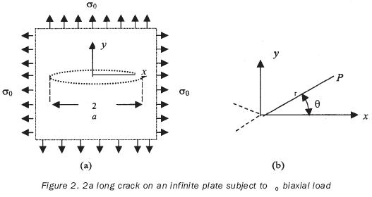
Elasticity problems involving elliptical or hyperbolic boundaries are dealt with using the elliptical coordinate system, figure 1. Thus:

where ξ > 0, 0 < η < 2 and –∞ < z < ∞ with c as a constant and scale factors defined by: h_ξ = h_η = a 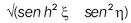and h_z=1. Figure 1 also shows the surface polar plots on plane XY. Eliminating η from the above equation:

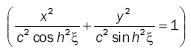
for the case ξ, = ξ,₀, the above equation is that of an ellipse whose major and minor axes are given by: a = c cosh ξ,₀ and b = c sinh ξ,₀.

Ellipse foci are x = ± c. The ellipse shape ratio varies as a function of ξ,₀. If ξ,₀ is very long and has a trend towards the infinite, the ellipse comes close to a circle with a = b. In addition, if ξ,₀ 0, the ellipse becomes a line 2c = 2a = 2b long, which represents a crack. This case is shown as part of the study on the intragranular fracture of a sample 16 µm long. Theoretically, an infinite plate with an elliptical micro discontinuity subject to a uniaxial load, figure 1a, should be taken into account to find that σ_η stresses around micro discontinuity are given by:

σ_{η =} σ₀ e^2ξ

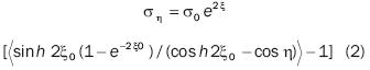
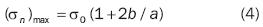
the boundary for stresses σ_η is a maximum at the end of the major axis, where cos 2η = 1. Replacing η in equation 2:

(σ_η) _max = σ₀ (1+ 2a / )b (3)

After examining the result of equation 3 for two limits, we find that when a=b or large ξ,₀, the elliptical microhole becomes circular and that (σ_η)_max = 3σ₀. This result confirms that stresses concentration for a circular microhole on an infinite plate with uniaxial load

may be described as:

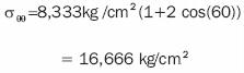
which represents σ₀₀ distribution around the micro discontinuity boundary for r = a.

The second result appears when b or ξ,₀=0 and the elliptical micro discontinuity spreads openly, showing a fracture. In this case, equation 3 proves that [σ_η] _max ∞ as b 0. It should be noticed that the maximum stress at the tip of the micro discontinuity at the end of the ellipse major axis tends towards the infinite, without considering the magnitude of the σ₀ applied stress, which shows that location takes place at the tip of the micro discontinuity for any load other than zero. When the σ₀ applied stress is parallel to the major axis of the elliptical micro discontinuity, figure 1b, the σ_η maximum value on the micro discontinuity boundary is the extreme point of the minor axis, and

At the limit when b 0 and when the ellipse represents a micro discontinuity, stress is (σ_n)_max = a₀. This does not apply at the extreme points of the micro discontinuity major axis, equation 4, but σ_v = – σ₀ for any b/a value. The theoretical solution for the plate elliptical micro discontinuity at the limit when b 0 proves distribution of stresses for the plate elliptical micro discontinuity. It is evident that stresses at the tip of the micro discontinuity are singular when the micro discontinuity is perpendicular to the σ₀ applied stress. The fact that stresses at the tip of the micro discontinuity are singular, shows that focal location takes place for any σ₀ stress other than zero and that predictive structural stability methods based on Tresca and Von Mises theories to locate them, are inappropriate.

 

Complex stress function for micro discontinuities

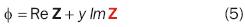
Let us now introduce a complex stress function, Z(z), pertaining to Airy stress function , given by:

as Z is a complex variable function, then:

Where z is defined as:

In order that Z is analytical in z₀, it must be defined in a z₀ environment, indefinitely derivable in the point given environment and must meet that given positive numbers δ and M, such as and that the following is true for any natural k number:

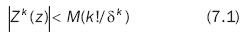
The analyticity criterion set by 7.1 is satisfactory as it may be determined in an absolute manner, but it is rather inconvenient in applications because it is based on knowledge of the behavior of any type of derivative in a certain environment, given the z₀ point.

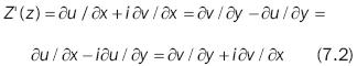
In order that Z satisfies analyticity on the area of interest, it must meet with the following: in order that a Z(z) = u(x, y) + jv(x, y) = φ(x, y) + j ψ (x, y) function defined in a G domain is derivable at z point of the domain as a complex variable function, and u(x, y) and v(x, y) functions must be able to be differentiated at this point (as functions of two actual variables) and the following conditions must be met at this point:

∂u / ∂x/ = ∂v ∂y & ∂u/ ∂y = –∂v / ∂x

If all the theorem conditions are met, the Z'(z) derivative may be expressed using one of the following forms, known as Cauchy–Riemann conditions¹ .

Transformation is 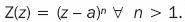This inequality transforms the extended plane on itself, so that each Z(z) point has n pre–images in the z plane. Thus:

with n points located on the apexes of a regular polygon with n sides and center point at a. The proposed transformation goes in accordance with all points, except z = a and z = ∞. In this case, the angles with apexes at the last two points increase n times. It should be taken into account that |Z(z) | = | z – a ⁿ | and that Arg (Z(z)) = n Arg(z – a), from which it may be deduced that every circumference with an a = b radius, figure 1, with center point atz = a is transformed into a circumference with an r radius. If point z displacing the | z – a| =r circumference in a positive direction, that is, the continually expanding Arg(z – a) increases by 2, a Z(z) point will displace n times the circumference defined by |Z(z) | =rⁿ in the same direction. The continually expanding Arg (Z(z)) will increase by 2n.

Now let us consider Joukowski's function (Kochin et al, 1958) Z(z) = ½ (z + 1/z) =λ (z), a second order function that meets the λ (z) = λ, (1/z) condition, which means that each point of the Z(z) plane has a Z(z) = λ (z) transformation of less than two z₁ and z₂, pre–images, related to each other by z₁z₂ = 1.

If one of them belongs to the inside of the unit circle, the other belongs to the outside and vice versa, while they have the same values. The Z(z) = λ (z) function remains in the domain and takes various values at the | z | < 1 (o | z | > 1) points, and is biunivocally and continuously transformed in a certain G domain of the Z(z) plane.

 

Theorem

The image of a γ unit circumference is the segment of the actual [–1,1] axis displaced twice (images of | z | = r circumferences and Argz = α + 2kradii), in such a manner that G domain is formed by every point of Z(z) plane, except for those belonging to the segment of the actual Γ axis meeting the values of the –1 < x < 1 interval.

 

Dem

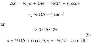
In order to obtain the domain's r boundary, the image of the γ : | z | = 1 unit circumference must be obtained. If , figure 2, then if

and the images of the | z | = r circumferences and the Argz = α + 2k radii

If we consider only the inside of the | z |< 1 unit circumference and the definition of z given in equation 7, that is:

then:

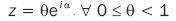
eliminating θ parameter we obtain:

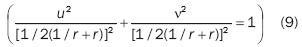
micro ellipse equation with

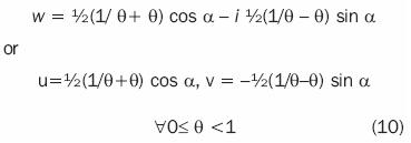
It may be inferred from equation 8 that when 9 increases continuously from 0 to 2or, which is the same, that point z traces the entire | z |= r circumference only once in a positive direction, the corresponding point traces the entire ellipse only once, represented by equation 9, in a negative direction. As a matter of fact, when 0 < θ < /2, u is positive and decreases from a down to 0, while v is negative and decreases from 0 down to –b. When / 2 < θ < , u continues decreasing from 0 down to –a, while v increases from–b up to 0. When < θ < 3 / 2, u increases from –a up to 0, while v increases from 0 up to b. Finally, when 3 / 2 < θ< 2 , u increases from 0 up to a, while v decreases from b up to 0.

If r radius of the | z | = r circumference varies from ∞ to 1, a is decreased from ∞ down to 1 and b is decreased from ∞ down to 0; the corresponding ellipses will trace the entire group of ellipses of w = Z(z) plane with ± 1 foci. From the above may be deduced that w = γ (z) transforms biunivocally the unit circle in the G domain representing the outside of the r segment. In addition, the image of the center of the unit circle is the infinite point and the image of the unit circumference is the Γ segment displaced twice.

For the image of the

radius, first we obtain the equation:

This shows that the images of two radii symmetrical to the actual axis (if α angle corresponds to one of them, –α angle are also symmetrical in relation to the actual axis; while the images of two radii symmetrical to the imaginary axis (if a angle corresponds to one of them, – α angle corresponds to the other one) are symmetrical to the imaginary axis. Therefore, it is only necessary to take into account the images of the radii belonging, for instance, to the first quadrant: 0 < α < /2.

It should be noticed that for α = 0, it is necessary that: This is an infinite semi–interval of the actual axis: 1 <  u < ∞. The interval that is symmetrical to this –∞ < u < –1, is the radius image corresponding to a = . For <  1. This is the imaginary semi–axis: – ∞ < v < 0. The other imaginary semi–axis 0 < v < ∞, is the radius image corresponding to a = – /2.

To summarize, the image of the unit circumference horizontal diameter is the infinite interval of the actual axis that goes from point –1 up to point + 1, passing through ∞; while the image of the unit circumference vertical diameter is the whole length of the imaginary axis, except for coordinates origin, including the infinite point.

Let us, now, suppose that θ < α < /2. If we eliminate the 6 parameter from equations in number 10, we obtain:

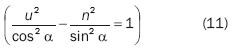
This is the equation of the hyperbola with actual semi–axis a = cos α, the imaginary semi–axis b = sin α and ± 1 foci. Nevertheless, point w does not completely trace the hyperbola when point z describes the whole length of 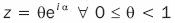radius. As a matter of fact, it might be deduced, based on equations in number 10, that when t increases from 0 up to 1, u decreases from ∞ down to cos α, while and v increases from –∞ to 0. Therefore, the point traces only a fourth of the hyperbola belonging to the fourth quadrant. Based on this observation, the fourth belonging to the first quadrant, i.e., the part symmetrical to the one given in relation to the actual axis, will be the image of the radius symmetrical to the given radius, in relation to the actual axis, i.e. of the radius corresponding to the –α angle. However, it would be unfair to say that the entire branch of the hyperbola that passes through the first and fourth quadrants is the image of the pair of radii referred to. In fact, the apex of hyperbola u = a, v = 0 does not belong to this image. The images of the radii corresponding to the – α and α + or α – angles are fourths of the same hyperbola, located in the third and second quadrants. The complete hyperbola, except its two apexes, is the image of the radii quatern: ± α, ± α. It must be noticed that the image of each of the diameters formed by these radii will be part of the hyperbola formed by the pairs of its fourths, which are symmetrical to the coordinates point of origin and that are interlinked at the infinite point.

To summarize, the w = λ (z) = ½ (z + 1/z) function biunivocally transforms both the inside and the outside of the unit circle on the outside of the second case –1 < u < 1 of the actual axis. The | z| = r circumferences are transformed into ellipses with ± 1 foci and similar (semi–axes): ½|1 /r ± r|, and the pairs of diameters symmetrical to the coordinate axes formed by radii 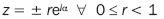are transformed into hyperbolas with ±1 foci and |cos α|, |sin α| semi–axes, except for the apexes of these hyperbolas.

Cauchy–Riemann conditions 7.2 lead us to:

This result proves that the Westergaard stress function automatically satisfies biharmonic equation: ⁴ = 0, which may be written as follows:

Highlighted functions and functions in bold type of the Z stress function in equation 5 indicate integration, i.e.:

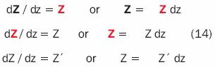
where bold type and the differential indicate integration and differentiation, respectively. If represent stress by a stress function such as:

where Ω (x, y) is a stress–body field.

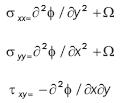
Substituting in equation 12, equations of stress Cartesian components are given in terms of the actual and imaginary parts of the Westergaard stress function:

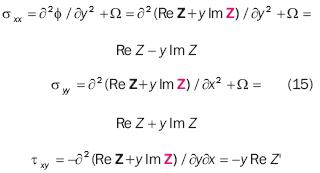
Equations in number 15 produce stress for Z(z) analytical functions. Besides, the stress function may be selected to meet the corresponding boundary conditions of the problem under study. The formula provided in number 15, originally proposed by Westergaard, relates correctly stress singularity to the tip of the crack. In addition, terms may be added to correctly represent the stress field in regions adjacent to the tip of the micro discontinuity. These additional terms may be introduced in later sections distributed with experimental methods to measure K_l.

The typical problem in fracture mechanics, figure 1a, is an infinite plate with a central crack 2a long. The plate is subject to biaxial stress. The Z stress function applied in order to solve this problem is:

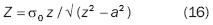
Substituting equation 16 in equation 15 for z ∞ , we obtain σ_xx = σ_yy and τ ' _{xy =} 0 and σ_xx = τ _xy = 0 as it is needed to meet the boundary conditions of the external field. On the discontinuity surface, where y = 0 and z = x, for –a < x < a, Re Z = 0 and σ_xx = τ _xy = 0. It is clear that the Z stress function given in equation 16 meets the boundary conditions on the surface free from micro discontinuities.

It is more convenient to relocate the point of origin of the coordinate system and the plate at the tip of the micro discontinuity, figure 2b. To translate the point of origin, z must be replaced in equation 16 by z + a, the new function being:

A small region near the tip of the micro discontinuity, where z << a, should then be taken into consideration. As a result, equation 17 is reduced to:

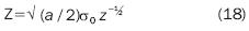
Substituting equation 6 in equation 18:

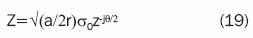
remembering that:

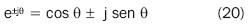
and replacing equation 20 in equation 19, it is proven that the actual part of Z is:

Along the line of the crack, where θ and y are both equal to zero, from 21 and 13:

This result proves that σ_yy ∞ stress is of a singular order as it gets closer to the tip of the micro discontinuity along the x axis. At last, equation 22 may be substituted in the following equation

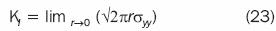
which is the treatment in the singular stress field introducing a known quantity as a stress intensity factor, K_l where the coordinate system shown in figure 2a and σ_yy is evaluated at the limit along the θ = 0 line. Therefore:

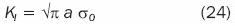
This result proves that K_I stress intensity factor varies as a lineal function of σ₀ applied stress and increases along with the length of the micro discontinuity as a function of , as shown in figure 3.

 

Application to laboratory tests

Usually, every theoretical solution to a physical problem must be proven in an experimental manner. That is why it is necessary to carry out laboratory tests in order to verify an analytical model. In this research, it is necessary to verify that the proposed solution model goes in accordance with observations carried out in the laboratory. The type of test was selected in accordance with ASTM E 399–90 (1993) test, which is used in order to determine the fracture resistance value on flat strain for metallic materials. During the preparation of samples was established a structural steel with a % thickness (1.905 cm). The type of material used complies with ASTM A–588 standard. Cutting and machining of samples were carried out by water and abrasive cutting with numerical control. Experimental design took into account a pilot sample in accordance with ASTM requirements, then the samples were instrumented and assayed after Dally y Riley's (1991) recommendations.

The four instrumented samples were assayed in accordance with that programmed in the experimental design, based on the pre–assay test. A metallographic treatment was carried out, which included: sample cutting, trimming and polishing with chemicals in order to make visible the microstructural features of the metal so that it could be subject to observation with digital scanning microscopy.

To apply the developed mathematical model, the elliptical and hyperbolic equations presented by micro discontinuities found during the microscopy session must be established. This has been possible generating a scale grid on the digital photographs obtained with the microscope, in order record the behavior of every micro discontinuity. Coordinates were recorded by scaling each photograph, tracing the contour of the micro discontinuity, placing a reference point of origin and tracing vertical and horizontal lines, depending on the shape of the micro discontinuity, at equal distances (similar to way a seismograph makes records), to read coordinates and create graphs using any type of spreadsheet, and determine the ideal equation for every micro discontinuity.

 

Ideal equations of various micro discontinuities

From all micro fractures observed in samples studied, it was decided to analyze those shown in figures 12 and 13 (Arteaga and Casanova, 2005), because they appear clearly in photographs. In figure 4, upper left corner, shows the generation of a micro discontinuity perpendicular to the horizontal fissure. This perpendicular micro discontinuity shows that its behavior coincides with the mathematical model shown in figure 1. The spreadsheet in figure 5 shows the tracing of these two micro discontinuities as well as the ideal behavior of the

ellipse (with dotted lines) governing the behavior of the lower micro discontinuity.

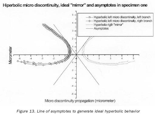
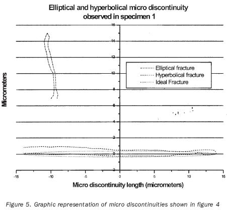
Figure 7 is the graphic representation of the image in figure 6. It was not possible to establish the ideal equation or behavior equation for this micro discontinuity, because its starting point coincides with the upper boundary of the notch, as shown in the figure. Therefore, it is not possible to obtain reference parameters, which renders it virtually impossible to establish their equation without resorting to a greater number of suppositions, which could lead to obtaining incorrect data regarding the behavior of such micro fracture.

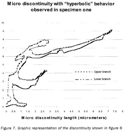
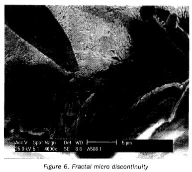
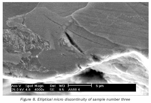
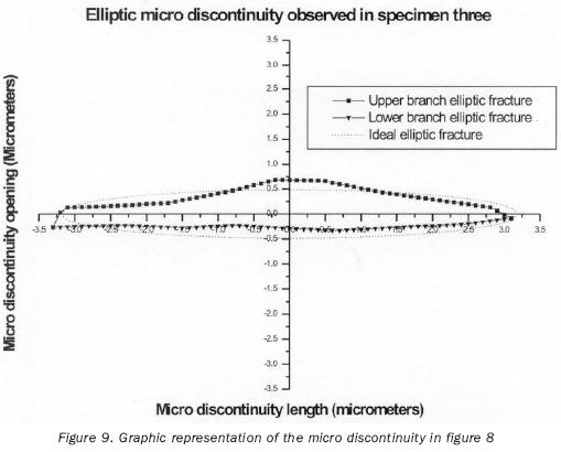
Figure 8 shows a micro fracture in sample number three, which has an elliptical behavior, while figure 9 shows its graphic representation. This micro fracture appeared on its own, without any hyperbolic behavior micro fractures. Figure 10 shows a series of micro fractures appearing in sample number one in an intergranular manner.

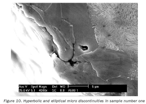
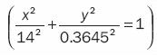
This figure shows generation of an elliptical micro fracture and the branches of hyperbolic micro fractures. Their ideal or particular equations were calculated, equations in number 15 were calculated afterwards. Figure 11 shows their graphic representation. On the other hand, figure 12 shows the left branch of the hyperbolic micro fracture, its ideal mirror, and the elliptical micro fracture and its ideal equation given by

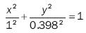
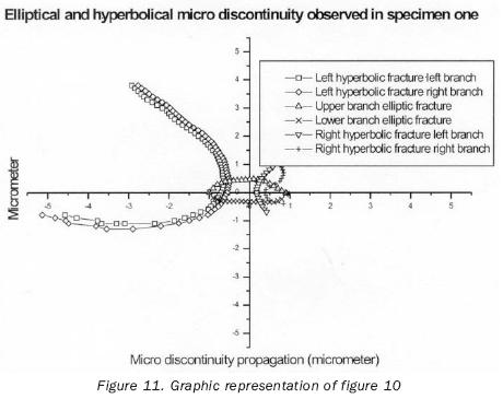
Figure 13 shows the hyperbolic micro discontinuity with its two branches, the ideal mirror and the line of asymptotes needed to establish the equation of such hyperbola. Finally, figure 14 shows the left branch of the hyperbolic micro discontinuity and the hyperbolic function graph representing the ideal behavior of the micro fracture accompanied by its asymptotes.

Calculation of stress on micro discontinuities in terms of the actual and imaginary parts of the Westergaard stress function, equation 15, uses equations obtained from the elliptical and hyperbolic representation of micro discontinuities shown in figure 10. Therefore, the equations of the ellipse and hyperbola to be transformed to the complex plane are, respectively:

 

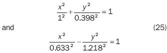
where a =1, b = 0.398 and c = 0.9174. The σ_x = σ₀ applied stress is:

 

The measured value of the r radius is equal to 0.79993, i.e.: a = b = 2.00083 * 0.398 = r.

 

Stress and actual stress intensity factors based on the complex variable model

To calculate the equation of the micro fracture, the following is substituted in equation 1:

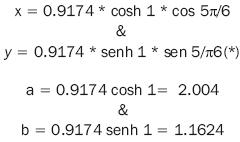
we must remember that ξ₀ = 1, is the starting point of the micro fracture and that the equation of the ellipse is:

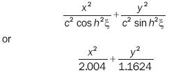
Theoretically, the σ_η stress around the micro–hole understudy is:

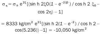
The σ_η stress boundary is a maximum at the end of the major axis when cos 2_η = 1; in this case: cos(10/6) = 0.5000106.

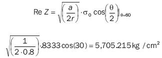
To calculate σ_θθ= σ_o(l + 2cos 20) radial stress, the value of the 0 angle on the upper branch has been measured directly from graph 12, this angle being 60°, thus:

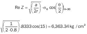
On the lower branch, θ value is 30°, thus:

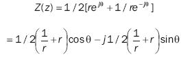
Therefore, the Z(z) function is:

For θ = 60°

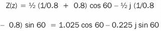
and the equation of the micro ellipse with semi–axes a = 1.025 and b = 0.225 is:

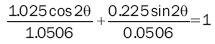
and

0.9756 cos²θ + 4.4466 sin² θ = 1

For θ =30°

Z(z) = 1.025 cos 30 – 0.225 j sin 30

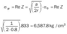
Equations for stress Cartesian components in terms of the actual and imaginary parts of the stress function are:

and

 

Along the line where θ and y are both zero, we obtain:

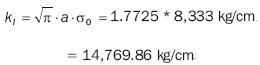
and its stress intensity factor is:

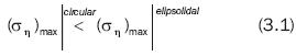
It must be noticed that, when observing figure 14 and comparing it with figure 1, becomes evident that a branch of the hyperbola has an angle such as that of the fracture under study, namely 60°, and that radial stress value is zero. This happens because when this hyperbola exists, the tip of the crack has disappeared and stress begins to be distributed over a much greater surface, leading to a decrease of such value and bringing about a change of sign. It may also be observed that, the smaller the hyperbola branch angle is, the greater the stress will be, which will tend to increase the closer the stress gets to zero (which means that it gets closer to the tip of the fracture), confirming the singularity of the stress at the tip of the fracture.

 

Conclusions

In micro fracture in figure 12 may be observed that the expansion of the crack at micrometric levels behaves in a fractal manner. Its equation is not presented. The distribution of particles close to the tip of the Chevron–type notch is circular in the well defined area of the plastic zone, which shows that the probe was subject to a high stress concentration. Applying the complex variable theory provides a complete view of the complexity of the theoretical problem involved. The w = λ (z) = ½ (z + 1/z) function transforms biunivocally both the inside and the outside of the unit circle on the outside of the second case –1 < u < 1 of the actual axis. It may be observed that, when there is a micro fracture that has already taken a hyperbolic shape and when the angle of some of its branches is 60° to the horizontal, the stress value is zero. Comparing the values of stress intensity factors taken at the laboratory and the theoretical results obtained, it may be ascertained that experimental values are the result of the overall effect of the test on the probe.

 

Acknowledgments

The authors want to thank research projects named Fractal and Fracture in Structural Samples No. 20040225 and No. 20050900. Financed by the Instituto Politécnico Nacional, Mexico.

 

References

Arteaga–Arcos, J.C and Casanova del Angel, F. (2005). Pruebas de laboratorio para el análisis de micro discontinuidades en acero estructural. El Portulano de la Ciencia. Año V, 1(14):543–558. House Logiciels. México.        [ Links ]

American Society of Testing Materials (ASTM) (1993). Standard E 813–89: Standard Test Method for Plane–Strain Fractures Toughness of Metallic Materials.        [ Links ]

Dally, J.Wand Riley W.F. Experimental Stress Analysis. McGraw–Hill. USA. 1991.        [ Links ]

Kochin N.E., Kibell A. and Rosé N.V. Hidrodinámica teórica. MIR. 1958.        [ Links ]

 

Suggesting biography

Anderson T.L. Fracture mechanics. CRC Press. USA. 1995.        [ Links ]

American Society of Testing Materials (ASTM) Standard E 399–90: Standard test method for plane–strain fractures toughness of metallic materials. 1993.        [ Links ]

Casanova del Angel F. La conceptualización matemática del pasado, el presente y el futuro de la arquitectura y su estructura fractal. El portulano de la ciencia, Año II, 1(4): 127–148, Mayo de 2003. 2001.        [ Links ]

Drexler E. Engines of creation. Anchor Books. USA. 1986.        [ Links ]

Juárez–Luna G. y Ayala–Millán A.G. Aplicación de la mecánica de fractura a problemas de la geotecnia. El portulano de la ciencia, Año III, 1(9):303–318. Enero de 2003.        [ Links ]

NASA. Fatigue crack growth computer program Nasgro versión 3.0. Referente Manual. Lyndon B. Johnson Space Center. USA. 2000.        [ Links ]

Regimex. Catálogo de productos. México. 1994.        [ Links ]

Gran Enciclopedia Salvat. Vols. 12 y 19. Salvat Editores S.A. Barcelona. 2000.        [ Links ]

Sears F.W. y Zemansky M.W. Física Universitaria. Vol. 1. Adison Wesley Longman–Pearson Education. México. 1999.        [ Links ]

Serway R.A. y Faughn J. S. Física. Prentice Hall–Pearson Education. México. 2001.        [ Links ]

Wilson J.D. Física. Segunda edición. Prentice Hall–Pearson Education. México. Capítulos 22 al 24. 1996.        [ Links ]

 

Notes

¹ This universally accepted denomination is historically unfair, as the conditions of 7.2 were studied in the 18th century by D'Alambert and Euler as part of their research on the application of complex variable functions in hydromechanics (D'Alambert and Euler), as well as in cartography and integral calculus (Euler).

 

About the authors

Francisco Casanova del Angel. Obtuvo el doctorado en estadística matemática en el año 1981, así como los estudios profesionales en estadística matemática en 1978 por la Université Pierre et Marie Curie, Paris VI. Asimismo, su maestría en ciencias en estructuras en 1974 en la Escuela Superior de Ingeniería y Arquitectura del IPN–México. Es licenciado en física y matemáticas desde el año de 1974 por la Escuela Superior de Física y Matemáticas del IPN–México. Fue asesor matemático de la Organización de las Naciones Unidas en 1981. Jefe de Departamento de Procesos y Métodos Cuantitativos de la Secretaría de Agricultura y Recursos Hidráulicos hasta 1985. Jefe del Departamento de Política y Gasto Paraestatal y Transferencia de la Secretaría de Agricultura y Recursos Hidráulicos hasta 1986. Subdirector de Procesos Estadísticos de la Secretaría de Turismo en 1987. Profesor del Instituto Politécnico Nacional desde 1971. Director General de Logiciels, SA de CV, desde 1985. Asesor Banco Mexicano SOMEX, SNC 1991–1992. Actualmente es responsable editorial de la revista científica "El Portulano de la Ciencia" y ha publicado un sin fin de libros y artículos en revistas de prestigio. Ha pertenecido a la Sociedad Mexicana Unificada de Egresados en Física y Matemáticas del IPN. Miembro de la Asociación Mexicana de Estadística. Miembro del International Statistical Institute. Miembro de la Classification Society of North America. Ha recibido diversas distinciones académicas y científicas como el Premio Nacional SERFIN El Medio Ambiente 1990, el Premio Excelencia Profesional 1998, la Medalla al Mérito Docente 2002, la Medalla Juan de Dios Bátiz 2002, el Premio a la Investigación en el Instituto Politécnico Nacional 2002, entre otros.

Juan Carlos Arteaga–Arcos. Civil engineer (IPN, 1995–2000), He postgraduate studies are M in S. with major in structures (IPN, 2001–.2005). Diploma: Desarrollo de proyectos de Innovación tecnológica (IPN, 2006), Ph Dr (candidate) with major in Advanced Technology (IPN, 2005–current). Someone congresses participation are: "Comportamiento mecánico de morteros de alta resistencia elaborados con cemento pórtland refinado" xv international material research congress, Cancún, Quintana Roo, México, august 20th to 24th, 2006. "Mechanical behavior and characterization of mortars based on portland cement processed by high–energy milling" 1st International Conference on Advanced Construction Materials, Monterrey, Nvo. León México, December 3rd to 6th, 2006. High energy ball milling as an alternative route to obtain ultrafine portalnd cement. 14th International Symposium on Metastable and Nano–Materials, Corfu, Greece, October 26th to 30th, 2007. High energy milling of portland–cement mortars precursors for enhacing its mechanical strength. 14th International Symposium on Metastable and Nano–Materials and "caracterizacion de cemento ultrafino obtenido a nivel laboratorio por molienda de alta energía" L Congreso Nacional de Física, Boca del Río, Veracruz, México, 29 de octubre al 2 de noviembre de 2007.