Educación en ingeniería

 

Solution of Rectangular Systems of Linear Equations Using Orthogonalization and Projection Matrices

 

La solución se sistemas rectangulares de ecuaciones lineales utilizando ortogonalización y matrices de proyección

 

M.A. Murray–Lasso

 

Department of Mechanical and Industrial Engineering Facultad de Ingeniería, UNAM, México
E–mail: mamurraylasso@yahoo.com

 

Recibido: julio de 2006
Aceptado: febrero de 2006

 

Abstract

In this paper a novel approach to the solution of rectangular systems of linear equations is presented. It starts with a homogeneous set of equations and through linear se space considerations obtains the solution by finding the null space of the coefficient matrix. To do this an orthogonal basis for the row space of the coefficient matrix is found and this basis is completed for the whole space using the Gram–Schmidt orthogonalization process. The non homogeneous case is handled by converting the problem into a homogeneous one, passing the right side vector to the left side, letting the components of the negative of the right side become the coefficients of and additional variable, solving the new system and at the end imposing the condition that the additional variable take a unit value.

It is shown that the null space of the coefficient matrix is intimately connected with orthogonal projection matrices which are easily constructed from the orthogonal basis using dyads. The paper treats the method introduced as an exact method when the original coefficients are rational and rational arithmetic is used. The analysis of the efficiency and numerical characteristics of the method is deferred to a future paper. Detailed numerical illustrative examples are provided in the paper and the use of the program Mathematica to perform the computations in rational arithmetic is illustrated.

Keywords: Rectangular systems of linear equations, Gram – Schmidt process, orthogonal projection matrices, linear vector spaces, dyads.

 

Resumen

En este artículo se presenta un nuevo enfoque para la solución de sistemas rectangulares de ecuaciones lineales. Comienza con un sistema de ecuaciones homogéneas y a través de consideraciones de espacios lineales obtiene la solución encontrando el espacio nulo de la matriz de coeficientes. Para lograrlo, se encuentra una base ortogonal para el espacio generado por las filas de la matriz de coeficientes y se completa la base para todo el espacio utilizando el proceso de Gram–Schmidt de ortogonalización. El caso no–homogéneo se maneja con virtiendo el problema en uno homogéneo, pasando el vector del lado derecho al lado izquierdo, usando sus componentes como coeficientes de una variable adicional y resolviendo el nuevo sistema e imponiendo al final la condición que la vari able adicional adopte un valor unitario.

Se muestra que el espacio nulo de la matriz de coeficientes está íntimamente asociado con las matrices de proyección ortogonal, las cuales se construyen con facilidad a partir de la base ortogonal utilizando díadas. El artículo maneja el método introducido como un método exacto cuando los coeficientes originales son racionales, utilizando aritmética racional. El análisis de la eficiencia y características numéricas del método se pospone para un futuro artículo. Se proporcionan ejemplos numéricos ilustrativos en detalle y se ilustra el uso del programa Mathematica para hacer los cálculos en aritmética racional.

Descriptores: Sistemas rectangulares de ecuaciones lineales, proceso de Gram–Schmidt, matrices de proyección ortogonal, espacios vectoriales lineales, díadas.

 

Introduction

The problem of solving a set of linear equations is central in both theoretical and applied mathematics because of the frequency with which it appears in theoretical considerations and applications. It appears in statistics, ordinary and partial differential equations, in several areas of physics, engineering, chemistry, biology, economics and other social sciences, among others. For this reason it has been studied by many mathematicians and practitioners of the different fields of application. Mathematicians of great fame such as Gauss, Cramer, Jordan, Hamilton, Cayley, Sylvester, Hilbert, Turing, Wilkinson and many others have made important contributions to the topic. Many numerical methods for the practical solution of simultaneaous linear equations have been deviced. (Westlake, 1968) Although some of them are reputedly better than others, this depends very much on the size and structure of the matrices that appear. For example, for very large matrices stemming from partial differential equations iterative methods are generally preferred over direct methods.

Although problems with square matrices are the ones most often treated, in this paper the problem with a rectangular matrix of coefficients is the target, the former one to be considered a particular case of the more general case.

 

The Homogeneous Case

Consider the following homogeneous system of m linear equations in n variables.

...............................................................(1)

which can be written in matrix form

...........................................................(2)

or more complactly

..................................................................................................(3)

In equations (1) and (2) the a_ij are rational numbers. Let us concentrate in the case m < n. Others are mentioned in the Final Remarks. If we consider the rows of matrix A in (2) as the representation with respect to a natural orthonormal basis of the form [1, 0, 0,..., 0], [0, 1, 0,..., 0],..., [0, 0,...0,1] of m n–dimensional vectors which span a subspace of Rⁿ, the domain of A, for which an inner product is defined by

......................................................(4)

What equation (2) is expressing is that the solution vector x must be orthogonal to the r–dimensional subspace spanned by the rows of matrix A, where r is the rank of matrix A which is equal to the number of linearly independent rows of A. From the theorem that states that (Bentley and Cooke, 1973).

...................................................................(5)

where R(A^T) is the range of the transpose of matrix A, and N(A) is the null space of A. We can deduce that the null space of A, which is the solution of equation (3), has dimension n–r and is orthogonal to the range of matrix A^T which is the subspace spanned by the rows of matrix A.

Hence, what we need to do to express the solution of equation (3) is to to characterize the subspace N(A). One way of doing this is to find a basis which spans it. From the theorem that states that for any inner product vector space (or subspace) for which we have a basis we can find an orthonormal basis for it through the Gram–Schmidt process (Bentley and Cooke, 1973). We intend to first find an orthonormal basis for the subspace spanned by the rows of matrix A using the Gramm–Schmidt process and then find its orthogonal complement obtaining therefore the solution subspace of equation (3). For this we will need orthogonal projection matrices which are easy to find when we have an orthonormal basis.

 

The Gram–Schmidt Process

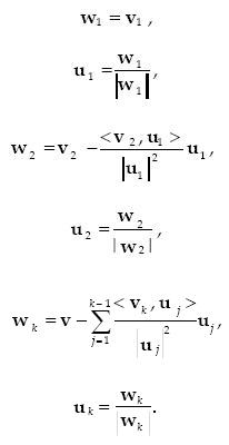
Given a set of r linearly independent vectors, the Gram – Schmidt Process finds recursively a sequence of orthogonal bases for the subspaces spanned by: the first; first and second; ... , first, second, ... , and r–th vectors. It accomplishes this by taking the first vector and using it as the first basis. It then takes the second vector and finds a vector that is orthogonal to the first by subtracting from the second vector its orthogonal projection on the first vector. The result is taken as the second vector of the orthogonal basis. This orthogonal basis spans the same subspace as the first two of the originally given linearly independent vectors. To get a third orthogonal vector the orthogonal projections of the third given vector upon the first two orthogonal vectors are subtracted from the third given vector. The result is orthogonal to both previous orthogonal vectors. The first three orthogonal vectors span the same subspace as the first three given vectors. The process is continued until all r given vectors are processed and an orthogonal basis for the r–dimensional subspace spanned by the given vectors is found. If it is desired to obtain an orthonormal basis, each of the orthogonal vectors can be normalized by dividing it by its length.

If we call w_i the i–th orthogonal vector of the final basis; u_i the i–th normalized orthogonal vector, and v_i the i–th given vector, the process can be described symbollically as follows:

...................................................................(6)

 

 

The Angular Brackett or Dirac Notation

In equations (6) and in the definition of the inner product we are using some aspects of a notation introduced by Dirac in his book on Quantum Mechanics (Dirac, 1947). We can think of vectors as row or column n–tuples which can be added and multiplied among themselves, as well as multiplied by scalars according to the rules governing matrices. We exhibit in equation (7) a sample of multiplication operations, recalling that matrix multiplication is non–commutative

................................(7)

We also recall that multiplication of a matrix by a scalar does commute and that the associative law is valid both for addition and multiplication of matrices.

In the Dirac notation a row matrix x is represented by the symbol < x, while a column matrix is represented by x >. (The row and column vectors do have significance in physical applications because they transform differently on changes of bases; they correspond to covariant and contravariant vectors and in some notations they are distinguished by making the indices super–indices or sub–indices). The inner product of two vectors corresponds to the first of equations (7) and is represented by <x, y>, a scalar, while the outer product of the same vectors (corresponding to the multiplication of a column matrix by a row matrix in that order) is represented by x><y which is an nxn matrix and corresponds to the second of equations (7). Notice that the matrix has rank equal to unity since all columns are multiples of the column vector (Friedman, 1956).

 

Dyads

The symbol x><y is a linear transformation (it is represented by a matrix) and so is the sum of several such symbols; they are called dyads, (when emphasis is put on the number of symbols involved it is sometimes called a one–term dyad or an n – term dyad.) Since we can think of a dyad as a matrix, it can be multiplied on the left by a row vector and on the right by a column vector, or multiplied either on the right or on the left by another dyad. Hence we have:

< z ( x > < y ) = ( < z, x > ) < y (a scalar multiplied by a row vector giving a row vector proportional to y.) It is usually written < z, x > y, ( x > < y ) z > = x > ( < y, z >) = ( < y, z >) x > (a scalar multiplied by a column vector giving a column vector proportional to x). It is usually written < y, z > x.

We used the property that scalars and matrices commute in multiplication. The results can be obtained by observing the way brackets open and close when terms are written in yuxtaposition. For this reason the symbol < is associated with the word "bra" while the symbol > is called "ket" and one looks for the appearance of the word "braket" to discover the presence of an inner product, while a "ketbra" corresponds to a dyad (Goertzel and Tralli, 1960).

Very often one uses an orthonormal basis to work with. When such is the case, an important formula that will be useful in the sequel is the following:

...............................................(8)

where u₁, u₂, ... , u_n are the orthonormal basis vectors for an n–dimensional inner product vector space and I_n is the unit operator for the n–dimensional space which is to be associated with an nxn unit matrix and maps each vector into itself. The va lidity of equation (8) can be verified by forming an orthogonal matrix Q with the u's as columns and multiplying it by its transpose Q^T and using the fact that the transpose of an orthogonal matrix is its inverse. and hence QQ^T = Q^TQ = I. The right hand side of (8) can be obtained by partitioning the matrix Q into submatrices that coincide with columns and the matrix Q^T into submatrices that coincide with rows as shown in equations (9).

...................................(9)

Equation (9) is called "the resolution of the identity" (Smirnov, 1970).

 

Orthogonal Projections

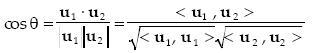
Whenever we use an orthonormal basis and represent vectors with n–tuples, the components of the n–tuples are the projections of the vector upon the coordinate axes whose orientations are those of the unit vectors of the basis. If we consider a vector as an arrow that goes from the origin of the coordinate system to the tip of the arrow, the projections coincide with the coordinates of the point located at the tip of the arrow. If we now take as basis the original basis rotated rigidly around the origin, leaving the arrow in its original position, the new n–tuple that represents the arrow has as components the projections of the arrow upon the new coordinate axes. Although in an n– dimensional space our intuition is not as good as in ordinary 2 or 3 dimensions, the inner product of vectors helps us to solve problems analytically. Extending concepts from 2 and 3 dimensions to n dimensions, we define the cosine of the angle θ between two vectors represented by n–tuples of coordinates in an orthonormal basis by the following formula

............................................(10)

To find the projection of the vector u₁ upon the line oriented in the direction of u₂ shown enhanced in Figure 1 we use the formula for the cosine of the angle between the two vectors given in equation (10) and obtain

...............................................(11)

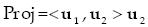
In the case that u₂ is a unit vector, its length is one and we can remove the denominator from equation (11). Additionally if we want the proyection to be a vector in the direction of u₂ we have

...............................................................................(12)

We have considered the projection of a vector upon an oriented line. One can also think of the projection of a vector upon a plane. A simple way of finding the projection of a vector upon a plane spanned by two ortho–normal vectors is to find the projections upon the orthonormal vectors and vectorially add them. The idea can be extended in a straight forward manner to more dimensions. Thus to find the proyection of a vector u upon a k–dimensional subspace spanned by orthonormal vectors v₁, v₂,...,v_k we can use the following expresion

...................................(13)

 

Orthogonal Projection Matrices

To solve the system of linear equations (3) we must characterize the null space of matrix A, which is the orthogonal complement of the space spanned by the its rows. The strategy we will use is to first find an orthonormal basis which spans the k–dimensional row space of A. For this purpose we utilize the Gram–Schmidt process for orthogonalizing the vectors represented by the rows of A. The set of orthonormal vectors thus obtained will span the same subspace as that spanned by the rows of A. The solution of the problem is the complementary subspace orthogonal to the one found. There are several possibilities for specifying this subspace. The simplest conceptually is to complete the orthonormal basis obtained with additional vectors to obtain an orthonormal basis for the n– dimensional space. This can always be done (Cullen, 1966). One way of doing it is to append to the rows of A a set of n linearly independent vectors and apply the Gram–Schmidt process to the complete set of vectors. A linearly independent set for the whole space which can be used for this purpose is the set {[1, 0, 0,..., 0], [0, 1, 0,..., 0], ... [0, 0, 0,..., 1]}. When applying the Gram–Schmidt process, if a vector is linearly dependent upon the previous vectors processed, the resulting vector will be the zero vector. The corresponding vector can be eliminated and the process continued with the rest of the vectors. If the rank of matrix A is k, then the first k vectors obtained in the process will span the space of the rows of A and the vectors k + 1, k + 2, ... , n will span the null space of A, the subspace sought. Each individual solution of equation (3) will then be an arbitrary linear combinations of these vectors. We now consider another approach based on orthogonal projection matrices.

We define an orthogonal projection matrix E as a idempotent symmetric square matrix, that satisfies the following two conditions: (Smirnov, 1970).

......................................................................................(14)

We now establish that the dyad v > < v, =1, is a projection matrix which can be expressed as a matrix V satisfying equations (14).

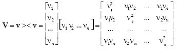
where we have applied the commutativity law to the scalars v_i, i = 1, 2,...n which are the components of v. The matrix is obviously symmetric by ispection. Additionally

...................(15)

In equation (15) we used the associativity law of matrices, the commutativity of the product of a scalar (the inner product) with a matrix and the fact that . This establishes that V is idempotent and therefore an orthogonal projection matrix.

According to equation (12) the matrix V transforms any column vector into its projection upon the vector v.

We now establish that the sum of r one–term dyads of the kind appearing in equation (15), where the vectors of the one–term dyads are the members of an orthonormal basis spanning a subspace R of dimension equal to the number of vectors in the basis, is also a projection matrix W that transforms any column vector into its projection upon the subspace R. To establish that the matrix is symmetric we proceed as before noting that the resultant matrix is the sum of symmetric matrices and is therefore symmetric. To establish idempotency we find the square of the matrix

When the mulyiplications are carried out, terms of the following nature are obtained

where we have commuted the inner product, which is a scalar with the vector on its left. If p≠q the inner product is zero, since it involves vectors which are orthogonal. If p= q then the inner product is unity since the vectors are normalized. Therefore only the terms squared remain and we obtain

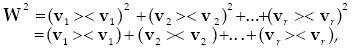
since according to equation (15) the terms squared are equal to the terms without the exponent, therefore

...............................................................................................(16)

and the two conditions establish W as an orthogonal projection matrix.

We now establish that the matrix I–W is an orthogonal projection matrix that maps any vector into its projection into the orthogonal complement sub space of the image subspace of W.

That I–W is symmetric is a consequence of the fact that both the unit matrix I and the matrix W are symmetric. Now let the n–dimensional space S be the domain of a linear transformation represented with respect to the natural basis {[ 1, 0 , ... , 0], [0, 1, ... , 0], ... [0, 0, ... , 1]} by a matrix A. The space S can be written as the direct sum of the subspace R spanned by the rows of A (the range of A^T) and the null space N of A (Zadeh and Desoer, 1963)

............................................................................................(17)

The subspace N is the orthogonal complement of R, hence every vector of R is orthogonal to every vector of N. Now suppose we have an orthonormal basis {v₁, v₂, ... ,v_n} such that the first r vectors span the row space of A and vectors r + 1, r + 2, ... , n span the null space of A. An arbitrary vector u can be written uniquely as the sum of two vectors, one in subspace R and the other in subspace N in terms of the orthonormal basis as follows:

If we call T the (n – k) – term dyad associated with the quantity enclosed by the second set of parentheses we get.

If we calculate T² we will find T = T² for the same reasons that in equation (16) we found that W² = W. We conclude that I – W is indeed an orthogonal projection matrix with the stated property of orthogonally projecting vectors in the domain of A unto the orthogonal complement of the row space of matrix A, that is, into the null space of A.

 

Back to the Homogeneous Linear Equations

Summing up, the method of solution of equation (3) using orthogonal projection matrices consists of finding orthonormal vectors v₁, v₂, ... , v_r, where r is the rank of matrix A that span the row space of A. This can be done using the Gram–Schmidt process. Next we form the matrix

The solution of equations (3) is the subspace given by

................................................................................................(18)

where y is an arbitrary vector in the domain of A.

A second method consists of finding an orthonormal basis for the domain of A by orthogonalizing a set of vectors formed by: first the rows of A appended with enough linearly independent vectors so that the set contains n linearly independent vectors. and orthogonalizing the set (discarding any zero vectors that may appear in the process) to obtain an orthonormal basis {v₁, v₂, ..., v_k, v_k+1, ... , v_n} for the domain of A. The solution of equations (3) is given by

...........................................................(19)

where c₁, c₂, ... , c_n are arbitrary scalars.

 

Numerical Illustrative Example

Consider the following homogeneous system of linear equations (Hildebrand, 1952)

.........................................................................(20)

The matrix A is therefore

.........................................................................(21)

The matrix is 3x4 and the rank of the matrix is 2, since the third row is equal to the second row minus the third. However, we will proceed as though we didn't know the third row is linearly dependent on the first two and let the process discover this fact.

We now proceed to orthogonalize the rows of A. Let the rows of A be a₁, a₂, a₃ and let q₁,... , q_r, where r is the rank of A, be the orthogonalized vectors. For numerical reasons it is more convenient not to normalize the vectors q_i in order to avoid taking square roots which might introduce unnecessary irrational numbers.

We take the first row as the first orthogonalized vector

The second orthogonalized vector is equal to the second row minus the projection of the second row on the first othogonalized vector, that is

We now seek the third orthogonalized vector which is equal to the third row minus the sum of its projections on the first and second orthogonalized vectors, that is

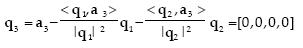
We have obtained the zero vector for the third orthogonalized vector. This shows that the third row of A is linearly dependent on the first two rows, thus the third row can be ignored and we have finished the orthogonalization process. The two vectors obtained (not normalized) are q₁ and q₂ . We can now find the matrix T.

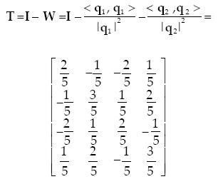
The solution to equations (20) is x_s = T y where y is an arbitrar y vector in the domain of A. For example if we choose y = [5, 0, 0, 0] we obtain the solution x_s = [2, –1, –2, 1]; while if we choose y = [0, 5, 0, 0] we obtain the solution x_s = ^..[–1, 3, 1, 2]. The reader can easily verify that both solutions satisfy equations (20). The two solutions obtained are linearly independent, therefore they span the two dimensional null space of matrix A, (the dimensionality of the null space of A coincides with the rank of matrix T and is also equal to n minus the rank of matrix A.) This means we can write the solution of equations (20) as an arbitrary linear combination of the two individual solutions found

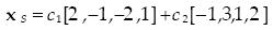...........................................................(2)

where c₁ and c₂ are arbitrary scalars.

We could also find the solution without resorting to projection matrices by finding two vectors linearly independent of the rows of matrix A and orthogonal to them. (The orthogonality is guaranteed for vectors that are transformed by matrix T). As we mentioned in the text, one possibility is to append candidate vectors to the rows of A and orthogonalize the whole set ignoring those vectors which give the zero vector. If the vectors a₄ = [1, 0, 0, 0], a₅ = [0, 1, 0, 0], a₆ = [0, 0, 1, 0] and a₇= [0, 0, 0, 1] are appended to the rows of A, we can guarantee that at least 4 vectors of the set {a_i}, i = 1, 2, ... , 7 are linearly independent. The orthogonalization would proceed in the same way as applied to the three rows of matrix A, its third row being deleted as before. The orthogonalization of the next vector a₄ = [1, 0, 0, 0] yields

Likewise q₄ would be

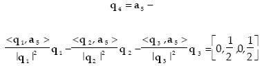
The reader can verify that q₁, q₂, q₃, q₄ are mutually orthogonal by checking that their inner products are zero when the indices are different. Once we have found four orthogonal vectors we can stop the process, since necessarily the last two vectors, being part of an orthonormal basis, will be linearly dependent with respect to the ones found. With q₃ and q₄ we can write the solution to equations (20) in the following manner

(The denominators in q₃ and q₄ can be incorporated into the c's becoming c primes and be eliminated). Although the solutions have some differences in appearance, the pairs of vectors span the same subspace so both solutions are equivalent.

There can be variations to the techniques applied. For example, instead of appending the elements of the natural basis and continuing the process of orthogonalization, we can start a new orthogonalization process for the null space in which additional vectors are obtained by multiplying T by arbitrary vectors y₁, y₂ obtaining vectors z₁, z₂. The first vector of the new orthogonalization process can be taken equal to z 1, the next one can be obtained by multiplying z ₂ by the matrix

The vector z₁ is guaranteed to be orthogonal to q₁ and q₂ and z₂ multiplied by U will be orthogonal to q₁, q₂, and z₁. We leave further details to the reader.

 

The Non–Homogeneous Case

So far we have considered only sets of equations with the right hand vector equal to zero. We now consider non – homogeneous systems of equations such as

.............................................................................................(23)

where A* is an m x (n – 1) matrix, x* is an (n – 1) – vector and b is an m – vector different from zero. This system can be converted to a homogeneous system by means of a simple trick. Subtract from both sides of the equation the vector b leaving zero in the right hand side and absorbing the vector – b on the left side as an additional column of matrix A* converting it to an m ft matrix A, adding a variable x_n to the vector x* to convert it into an n–vector x and changing the system to a homogeneous system of the form of equation (3).

.................................................................................................(3)

Equations (23) and (3) are equivalent if to equation (3) we add the restriction x n = 1, a condition that can be imposed after the solution of (3) has been obtained. To obtain the solution of equation (3) we apply the methods that have been given in the paper. Equation (3) always has a solution (the zero vector is always a solution) while equation (23) may not have a solution; this situation arises when it is not possible to apply the condition x_n = 1 at the end, which can happen if all solutions of equation (3) give values to x_n different from 1, making it impossible to apply the restriction required.

 

Illustrative Example of a Non –Homogeneous System of Equations

Consider the following system of linear equations (Hadley, 1969).

..............................................................................(24)

Equations (24) have the unique solution x₁ = 1, x₂ = 2, x ₃ = 3. This can be obtained easily by using Cramer's Rule. The augmented matrix of the system is

...........................................................................(25)

We will use rational arithmetic to obtain exact results with the aid of the program Mathematica (Wolfram, 1991). The instructions in Mathematica for the necessary calculations are:

The assignment operator in Mathematica is : = . Notice that rectangular matrices are provided to the program as a list of lists, each list is enclosed in braces. Vectors are provided as a single list enclosed in braces. a[[i]] denotes the i – th row of matrix a. Inner products of vectors and as well as the product of rectangular matrices is indicated by a dot between the operands. The addition or subtraction of matrices uses the operators "+" and "–" between the matrices. Products of scalars and vectors or matrices are indicated by yuxta– position. A dyad vec1><vec2 can be constructed using the function Outer [Times, vec1, vec2] and the result is a square matrix. A unit matrix of order n is generated by the function IdentityMatrix[n]. Division between two scalars uses the symbol /.

When 15T is written in the conventional manner we have

Absorving the factor 15 into the arbitrary vector y when we multiply T by y we obtain an answer x_s which is always a multiple of the vector [1, 2, 3, 1] (This is due to the fact that all columns of T are multiples of this vector, since T has rank 1), therefore

By choosing k = 1 we satisfy the condition that x_n = 1, hence the unique solution to equations (24) is the vector [1, 2, 3].

 

Final Remarks

We have given a novel method for solving rectangular homogeneous systems of linear equations. The method is based on applying the Gram–Schmidt process of orthogonalization to the rows of the matrix and either calculating an orthogonal projection matrix and multiplying it by an arbitrary vector, or continuing the orthogonalization process to calculate a basis for the null space of the matrix of coeficients of the original system from which a general solution to the problem is obtained. Although in the paper the discussion was carried out as though the matrix of coefficients had less rows than columns, what is important is the rank of the matrix and the number of variables (dimension of the domain space). Since a homogeneous system always satisfies the trivial zero solution, there arises no question relative to the existance or not of a solution. If the rank r of the matrix is equal to the dimension n of the domain, the zero solution is the only solution, otherwise the rank is less than the dimension of the domain and the solution is the null space of the matrix of coefficients. This null space has dimension n – r. To handle non– homogeneous systems of equations the paper gives a simple trick for converting the problem into an equivalent homogeneous problem whose domain has a dimension larger than the original by one unit. Illustrative numerical examples are given in the paper.

No discussion of the numerical properties of the method nor of its computational efficiency compared to other methods is given in the paper, this is left for a future paper. The illustrative examples are solved exactly using rational arithmetic, thus no approximations are used. The use of the program Mathematica as an aid in the calculations in rational arithmetic is exhibited in one of the illustrations and the actual instructions are shown together with results.

 

References

Bentley D.L. and Cooke K.L. (1973). Linear Algebra with Differential Equations. Holt, Rinehart and Winston, Inc., New York.        [ Links ]

Cullen C. (1966). Matrices and Linear Transformations. Addison–Wesley Publishing Company, Reading, MA.        [ Links ]

Dirac P.A.M. (1947). The Principles of Quantum Mechanics. Third Edition, Oxford Uiversity Press, New York.        [ Links ]

Friedman B. (1956). Principles and Techniques of Applied Mathematics. John Wiley & Sons, Inc., New York.        [ Links ]

Goertzel G. and Tralli N. (1960). Some Math e matical Methods of Physics. McGraw–Hill Book Company, Inc., New York.        [ Links ]

Hadley G. (1969). Álgebra lineal. Fondo Educativo Interamericano, S.A., Bogotá.        [ Links ]

Hildebrand F.B. (1952). Methods of Applied Mathematics. Prentice–Hall, Inc., Englewood Cliffs, NJ.        [ Links ]

Smirnov V.I. (1970). Linear Algebra and Group Theory. Dover Publications, Inc., New York.        [ Links ]

Westlake J.R. (1968). A Handbook of Numer ical Matrix Inversion and Solution of Linear Equations. John Wiley & Sons, Inc., New York.        [ Links ]

Wolfram S. (1991). Mathematica: A System for Doing Mathematics by Computer, Second Edition. Addison–Wesley Publishing Company, Inc., Redwood City, CA.        [ Links ]

Zadeh L.A. y Desoer C.A. (1963). Linear System Theory: The State Space Approach. McGraw–Hill Book Company, Inc., New York.        [ Links ]

 

Semblanza del autor

Marco Antonio Murray–Lasso. Realizó la licenciatura en ingeniería mecánica–eléctrica en la Facultad de Ingeniería de la UNAM. El Instituto de Tecnología de Massachussetts (MIT) le otorgó los grados de maestro en ciencias en ingeniería eléctrica y doctor en ciencias cibernéticas. En México, ha laborado como investigador en el Instituto de Ingeniería y como profesor en la Facultad de Ingeniería (UNAM) durante 45 años; en el extranjero, ha sido asesor de la NASA en diseño de circuitos por computadora para aplicaciones espaciales, investigador en los Laboratorios Bell, así como profesor de la Universidad Case Western Reserve y Newark College of Engineering, en los Estados Unidos. Fue el presidente fundador de la Academia Nacional de Ingeniería de México; vicepresidente y pres i dente del Consejo de Academias de Ingeniería y Ciencias Tecnológicas (organización mundial con sede en Washington que agrupa las Academias Nacionales de Ingeniería) y secretario de la Academia Mexicana de Ciencias. Actualmente es jefe de la Unidad de Enseñanza Auxiliada por Computadora del Departamento de Ingeniería de Sistemas, División de Ingeniería Mecánica e Industrial de la Facultad de Ingeniería de la UNAM. Miembro de honor de la Academia de Ingeniería y de la Academia Mexicana de Ciencias, Artes, Tecnología y Humanidades.