


Serviços Personalizados
Journal
Artigo
 Inglês (pdf)
 Artigo em XML
 Referências do artigo
 Enviar este artigo por email
Indicadores
-
 Citado por SciELO
 -
 Acessos
Links relacionados
-
 Similares em
SciELO
Similares em
SciELO
Compartilhar

 Permalink
Ingeniería, investigación y tecnología
versão On-line ISSN 2594-0732versão impressa ISSN 1405-7743
Ing. invest. y tecnol. vol.8 no.3 Ciudad de México Jul./Set. 2007
Educación en ingeniería
Practical Design of Digital Filters Using the Pascal Matrix
B. Psenicka1, F. García–Ugalde 2 and V.F. Ruiz3
1 Department of Telecommunications, Facultad de Ingeniería, UNAM
E–mail: pseboh@servidor.unam.mx
2 Department of Digital Signal Processing, Facultad de Ingeniería, UNAM
E–mail: fgarciau@servidor.unam.mx
3 Department of Cybernetics, The University of Reading, Reading RG6 6AY, UK.
E–mail: v.f.ruiz@reading.ac.uk
Recibido: julio de 2006
Aceptado: abril de 2007
Abstract
In the context of the design of digital filters many research has been done to facilitate their computation. The Pascal matrix recently defined in (Biolkova and Biolek, 1999) has proved its utility in this field. In this paper we summarize the direct transform from the lowpass continuous–time transfer function H(s) to the discrete–time H(z) of the following main tree types of digital filters: lowpass, highpass and bandpass. An alternative representation of the original bandpass Pascal matrix is de veloped in this paper that permits to convert systematically the lowpass continuous–time prototype to the discrete–time bandpass transfer function. We also consider the inverse transformation from the dis crete–time domain to the continuous one and we show that the inverse transformation is easily obtained as the determinant of the system need not to be com puted. Several numerical examples illustrate the practical utilization of this technique.
Keywords: Filter design, s–z transformation, Pascal matrix, digital filter design tools.
Resumen
En el contexto del diseño de filtros digitales se ha desarrollado mucha investigación para facilitar su cálculo. La matriz de Pascal definida recientemente (Biolkova and Biolek, 1999) ha probado su utilidad en este campo. En este artículo se hace una síntesis de la transformación directa a partir de la función de transferencia pasa–bajas en tiempo continuo H(s) para obtener la de tiempo discreto H(z) de cada uno de los tres tipos principales de filtros digitales: pasa–bajas, pasa–altas y pasa–banda. También se desarrolla una representación alternativa de la matriz de Pascal pasa–banda original, que permite la conversión sistemática de un prototipo pasa–bajas en tiempo continuo a la función de transferencia pasa–banda en tiempo discreto. Adicionalmente se considera la transformación inversa a partir del dominio de tiempo discreto, al de tiempo continuo y se demuestra que esta transformación inversa es fácil de calcular, dado que no es necesario obtener el determinante del sistema. Varios ejemplos numéricos ilustran la utilización práctica de esta técnica.
Descriptores: Diseño de filtros, transformaciones s–z, matriz de Pascal, herramientas para el diseño de filtros digitales.
Introduction
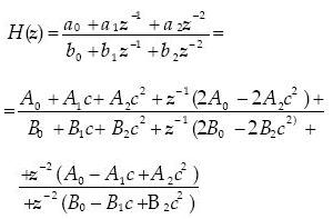
A large number of procedures are available for designing digital filters (Parks and Burrus, 1987); (Antoniou, 1993). Many of them transform a given analog filter into an equivalent digital filter. The digital filter design process begins with the synthesis or specification of the filter transfer function. A signal x(t) presented to a filter characterized by its impulse response h(t) produces an output y(t) given by the convolution y(t)=x(t)*h(t) or, if using the continuous–time transforms of the signals, by Y(s)=X(s)H(s). Then the continuous–time circuit of a filter is completely described by the transfer function:
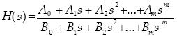 .........................................................(1)
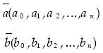
From this equation the vectors  and
and  representing respectively the coefficients of the numerator and denominator can be defined as:
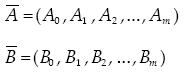 .......................................................................(2)
where, Ai and Bi are real coefficients.
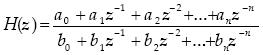
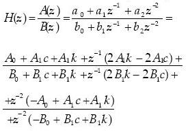
In the discrete–time domain the z transforms of the signals are used, and a digital filter is characterized by the transfer function:
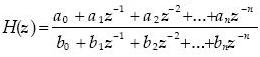 ........................................................(3)
With real coefficients ai and bi .
The problem of the systematic conversion from the continuous–time prototype transfer function H(s) to its discrete–time version H(z) is addressed in this paper considering three types of conversions: lowpass–to–lowpass, low–pass–to–highpass and lowpass–to–bandpass. The original Pascal matrix (Biolkova and Biolek, 1999) is used to achieve this systematization, and an alternative representation of the original Pascal matrix is developed in this paper to rich the lowpass–to–bandpass conversion.
The remainder of this paper is organized as follows. Section II describes the lowpass–to–lowpass conversion. Section III adapts the previous development to the lowpass–to–highpass case. Section IV main contribution of this paper, develops an alternative representation of the original bandpass Pascal matrix which allows the lowpass–to–bandpass conversion. Section V presents the inverse conversion from the discrete–time domain to the continuous–time. In Section VI we give examples to illustrate all the cases.
Lowpass–to–lowpass Transformation
For lowpass filters the digital transfer function H(z) can be obtained from the continuous–time prototype (1) using the bilinear s–z transformation (Parks and Burrus, 1987):
 .............................................................................................(4)
where
 ...........................................................................................(5)
and the constants f1 and f2 represent the lowpass corner and sampling frequencies, respectively.
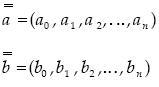
From the transfer function (3), we define the vectors  and
and  whose elements are respectively the coefficients of the numerator and denominator (Klein, 1976):
 ............................................................................(6)
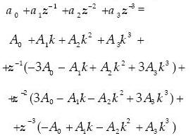
In order toexpress the numerator vectors in terms of and denominator vectors in terms of , we replace the variable s in (1) by (4) then comparing the numerators and the denominators of the resulting transfer functions in z, we can identify the coefficients by equating the coefficients of the like powers in z.
Thus, for n=2 and m=2 we obtain the following expression:
 ................................................(7)
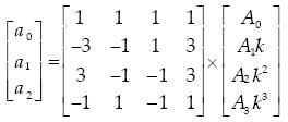
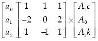
From the numerators the coefficients, ai, i=0,1,2 are easily identified and re–written in acquire the following matrix equation
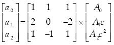 ...............................................................(8)
In a similar manner, a matrix equation can be obtained for the coefficients, bi, i=0,1,2 of the denominator vector .
Using a more compact representation both equations can be written as follows:
 .........................................................................................(9)
where  is the lowpass Pascal matrix defined_in_(Psenicka et al., 2002) and the vectors
  ,
,  are represented by
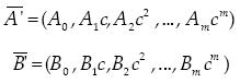 .................................................................(10)
As demonstrated in (Psenicka et al., 2002) the computation of the matrix can be done in a systematic form. For this we consider the classical Pascal Triangle
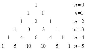 .....................................................(11)
Observe, that the coefficients of base n=2 create the last column in the lowpass Pascal matrix of (8) with the exception of the elements in the even rows which have negative values. We have concluded that the lowpass Pascal matrix can be formed by taking into account the following rules (Biolkova and Biolek, 1999); (Pham and Psenicka, 1985).
– In the first row of the Pascal matrix all the elements must be equal to one.
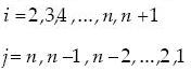
– The elements of the last column can be computed using:
.....................................................(12)
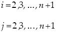
where
i=1,2,...,n+1
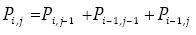
The remaining elements Pi,j of the lowpass Pascal matrix can be determined using the following equation:
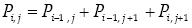 ......................................................................(13)
where
Without lost of generality, using letters of the alphabet in the order shown below we can identify the elements of the lowpass Pascal matrix for n=4:
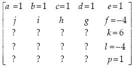 .......................................................(14)
where the elements denoted g, h, i, and j can be obtained using the next set of equations:
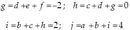 ........................................................(15)
Then the lowpass Pascal matrix for the particular case of n=4 is finally given by:
 ...............................................................(16)
Lowpass–to–highpass Transformation
In this second case, in order to transform the lowpass transfer function to the discrete highpass transfer function H(z), we substitute the variable s by 1/s in (4). Thus,

with
 ...........................................................................................(17)
where fc represents the cut–off frequency of the highpass and fs the sampling frequency. Following the same process, substituting (17) into (1) and comparing the numerator with (3) for n=3 and m=3, we can obtain:
 .....................................................(18)
Again, equating the coefficients of the like powers in z, we obtain the following matrix equation
 .......................................................(19)
This equation can be written in the compact form
 ........................................................................................(20)
where  is a variant of a Pascal matrix which corresponds to the highpass filter in which the first row elements are all equal to one, and the elements of the first column can be obtained using (12). The remaining elements Pi,j can be determined using the following expression (Psenicka et al., 2002):
 .....................................................................(21)
Where
A similar development can be done for the denominator vector .
Lowpass–to–bandpass Transformation
The latest case considered in this paper shows how to obtain a discrete bandpass filter (Konopacki, 2005) characterized by the discrete–time transfer function H(z)
 .......................................................(22)
which also has real coefficients ai and bi. As previously this transfer function can be obtained from the continuous one (1) by s–z transformation. The bandpass filter can be seen as a superposition of a lowpass filter and a highpass filter (Rabiner and Gold, 1975). Thus, the s–z transformation that applies is (Bose, 1985):
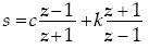 .................................................................................(23)
where
f1 and f–1 represent the upper and lower frequencies of the bandpass filter respectively, and fsthe sampling frequency.
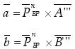
In a similar manner from (22), we define the coefficient vectors and :
 ...............................................................................(24)
In order to obtain the coefficients ai and bi (i =0,1,...,n) knowing the continuous time representation vectors and , we must first substitute (23) into (1) then compare the numerator and denominator of the resulting transfer function with the corresponding ones in (22).
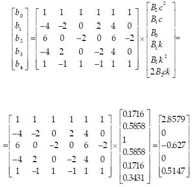
For example without lost of generalization we take m=1 in (1), due to the high order terms appearing in the transformation (23), a n=2 must taken in (22) resulting in:
 ....................................................(25)
and the following matrix equation:
 ....................................................................(26)
A similar equation is obtained for the denominator vector . Both equations can be represented in the following compact form:
 .......................................................................................(27)
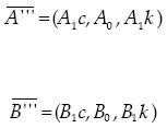
where  is the so called bandpass Pascal matrix. This matrix transforms the normalized lowpass to bandpass transfer function. We have named this matrix the bandpass Pascal matrix (Psenicka and García–Ugalde, 2004) because the matrices of all orders have in the first column the coefficients of the base of a Pascal triangle (11) with the exception of elements in even rows, which have negative signs. In this example the vectors
  and
and  are represented respectively by
 ..............................................................................(28)
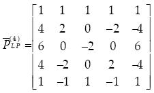
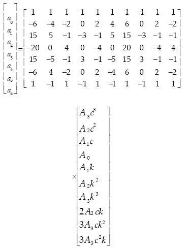
In order to achieve an alternative representation of the original bandpass Pascal matrix, without lost of generality let us consider the case of order m=2 and again because of the high order terms appearing in the transformation (23), a n=4 must taken. The matrix representation 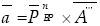 is given by
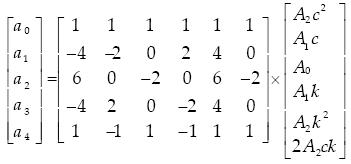 ......................................(29)
Note from this latest example that the matrix is rectangular and it will be the general case in a lowpass–to–bandpass transformation for values of m=2 or higher. In order to use the same rules as in the previous section for the lowpass–to–highpass transformation (which always has a square matrix) we decompose this rectangular matrix into the concatenation of two matrices as shown in the following equation
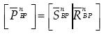 ...............................................................................(30)
In this equation the matrix  is square and its computation is exactly the same as that used in the lowpass–to–highpass transformation, which means: all the terms in the first column can be obtained using (12) and the remaining elements Sij can be established using the following expression (PseniUka et al., 2002):
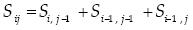 .....................................................................(31)
Where
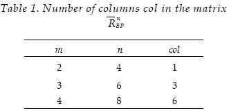
On the other hand the matrix  in (30) is rectangular with n+1 rows. A priori the number of columns has to be computed by counting the number of elements different to 1 included in the upper triangle from base m of the Pascal triangle (11). To illustrate these values we summarize in table 1 the number of columns col of matrix for different m and n parameter values.
Once the elements of matrix  are known the columns of
  can be derived directly. Let us consider the case m=2, the lonely column of is equal to the central column of (Psenicka and García–Ugalde, 2004). In this paper we call this column the pivot because for m=2 there is only one element different to 1 in the upper triangle from base m in the Pascal triangle and its position corresponds to a central position in the triangle. For m=3, as shown in table 1, there are three columns in , one is also the pivot because again it is equal to the central column of and the two others are the columns on the right of the pivot and on the left of it. Also the reason is because for m=3 there are three elements different to one in the upper trian– gle from base m and their positions corres– pond to a central position in the triangle plus its nearest neighbors (right and left). To illustrate the previous structure we show the resulting
  matrix for vector and parameters m=3, n=6.
 ...................................(32)
A similar expression can be obtained for vector .
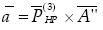
Inverse Transformation from H(z) to H(s)
The inverse Pascal matrix is defined by the following equation (Klein, 1976):
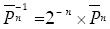 .......................................................................................(33)
In all cases using the inverse Pascal matrix the continuous–time transfer function H(s) can be obtained from the transfer matrix of the discrete–time structure H(z). The advantage of using this equation is that to compute the inverse Pascal matrix the determinant of the system is not necessary.
For example consider the lowpass case, let H(z) be the transfer function of the discrete structure that works at the corner frequency
f1 = 3400[Hz] and sampling frequency
fs= 16000 [Hz].
 .........................................................(34)
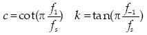
First it is necessary to calculate the constant c of the bilinear transform (1):
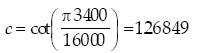 .....................................................................(35)
Then the transfer function coefficients of the analog circuit will be calculated as follows:
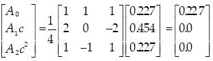 ..............................................(36)
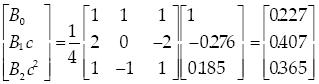 ............................................(37)
and
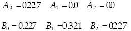
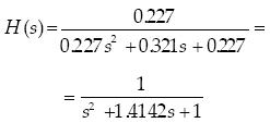
The transfer function of the corresponding analog filter is the Butterworth transfer function of the second order:
Numerical Exam ples
In these examples we shall transform a lowpass transfer function H(s) to lowpass and highpass transfer functions H(z) using the features specified by:
 ...............................................(38)
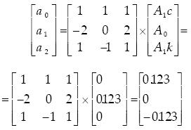
Transformation LP–to–LP from s to the z domain
The transfer function coefficients ai ,bi, for i=0,1,2,3 can then be obtained using the equations:
 .....................................................(39)
 .......................................................(40)
given
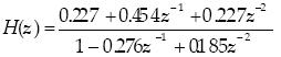
The transfer function H(z) takes the form
 ...........................................(41)
For this equation the corresponding magnitude and phase frequency responses of the digital lowpass filter are shown in Figure 1.
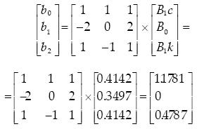
Transformation LP–to–HP from s to the z domain
Using the Pascal matrix  we can transform the lowpass transfer function (38) to the highpass transfer function H(z) using the following equations:
 ......................................................(42)
 .................................................(43)
The coefficients of the highpass transfer function are:
and the highpass transfer function is given by (44). The magnitude and phase frequency responses of the digital highpass filter are shown in Figure 2.
 ...........................................(44)
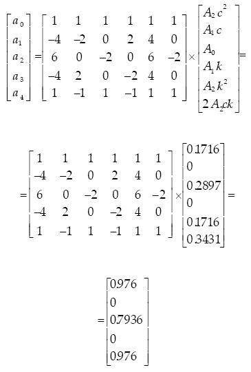
Transformation LP–to–BP from s to the z domain
In this example we transform a Butterworth lowpass transfer function H(s) to a bandpass transfer function H(z) using the features specified by:
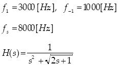 .............................................................(45)
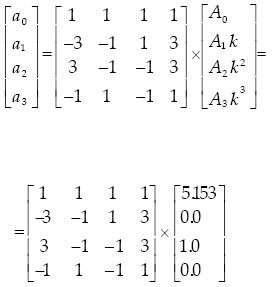
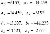
In order to transform the lowpass analog function (45) into the digital bandpass function, we must first determine the transfer function coefficients a1,b1 for i=0,1,...,4 which can be obtained using the matrix equations for current values:
 ...................................(46)
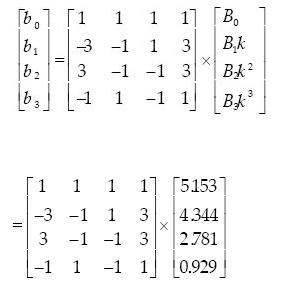
 ............................(47)
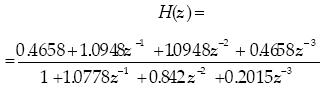
The transfer function of the bandpass filter is given by
 ..........................................................(48)
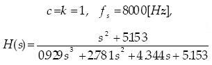
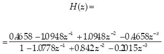
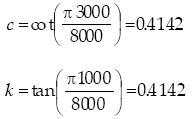
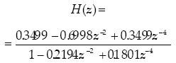
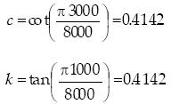
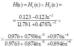
Finally, a more complicated example is presented, in which the lowpass transfer function H(s) contains two transfer functions H1(s) and H2(s) and is transformed into the whole system bandpass transfer function H(z) for f1=3000[Hz], f–1=1000[Hz], fs=8000[Hz]
 .........................................................(49)
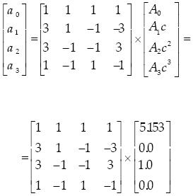
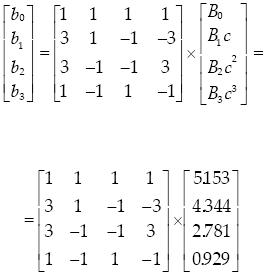
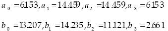
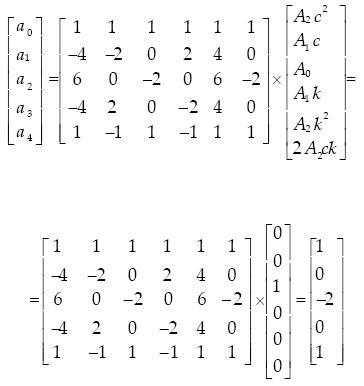
In order to transform the lowpass analog function (49) into the digital bandpass function, we proceed the s–z transformation for each of these two transfer functions, we must first establish the coefficients ai,bi, for i = 0,1,2 for the first function H1(z) and then the coefficients ai, bi, for i=0,1,2,.. .,4 for the second one H2(z). This computation can be obtained using the matrix equations previously defined for current values:
 ......................................................(50)
 ....................................................(51)
 ...................................(52)
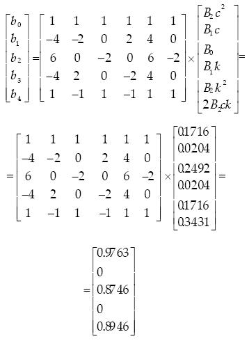 .....................................(53)
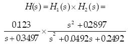
The whole system transfer function in z of the bandpass filter is given in (54) and the corresponding magnitude and phase frequency responses are shown in Figure 3.
 ............................................................(54)
Conclusions
The Pascal matrix is very useful in the context of the design of digital filters. Transformations can easily be done from the analog prototype lowpass transfer function H(s) to the discrete transfer function H(z) to obtain one of the main three types of digital filters: lowpass, highpass and bandpass. The inverse transformation from discrete to analog is very easy to achieve as well because we do not need to compute the determinant of the system. In this paper we have summarized all types of direct transformations and illustrate their use with several numerical examples. An alternative representation of the original bandpass Pascal matrix has been presented for the systematic computation of the bandpass Pascal matrix.
Acknowledgements
This research was supported by CONACyT México, project 41069–Y and DGAPA–UNAM, project IN101305.
References
Antoniou A. (1993). Digital Filters: Analysis, Design, and Applications. McGraw–Hill, New York, USA. [ Links ]
Biolkova V. and Biolek D. (1999). Generalized Pascal Matrix of First Order s–z. Trans forms. ICECS, Pafos, Cyprus, Vol. 2, pp. 929–931, September. [ Links ]
Bose N.K. (1985). Digital Filters Theory and Applications. Elsevier Science Publishing Co., Inc., Amsterdam, The Netherlands. [ Links ]
Klein W. (1976). Finite Systemtheorie. B.G. Teubner Studienbücher, Stuttgart. [ Links ]
Konopacki J. (2005). The frequency Trans formation by Matrix Operation ans its Application in iir Filters Design. IEEE Signal Processing Letters, Vol. 12, No. 1, pp. 5–8, January. [ Links ]
Parks T.W. and Burrus C. (1987). Digital Filter Design. John Willey and Sons, Inc., New York, USA. [ Links ]
Pham Khac di and PseniUka B. (1985). Transfer Function Computation Using Pascal Matrix. Electronic Horizon–Praha, Vol 46–7, pp. 348–350. [ Links ]
Psenicka B. and García–Ugalde F. (2004). Z–transform from Lowpass to Bandpass by Pascal Matrix. IEEE Signal Processing Letters, Vol. 11, No. 2, pp. 282–284, February. [ Links ]
Psenicka B., García–Ugalde F. and Herrera–Camacho A. (2002). Z–transfromation from Lowpass to Lowpass and Highpass Transfer Function. IEEE Signal Processing Letters, Vol. 9, No. 11, pp. 368–370, November. [ Links ]
Rabiner R. and Gold B. (1975). Theory and Applications of Digital Signal Processing. Prentice–Hall, New Jersey, USA. [ Links ]
Suggesting Biography
Bellanger M. (2000). Digital Processing of Signals, Theory and Practice. John Willey and Sons, Inc., Chichester, UK.
Manolakis D.G. and Proakis J.G. (1996). Digital Signal Processing: Principles, Algorithms, and Applications. Prentice–Hall, New Jersey, USA.
Mitra S.K. and Kaiser J.F. (1993). Handbook of Digital Signal Processing. John Willey and Sons, Inc., New York, USA.
Oppenheim A.V. and Schafer R.W. (1975). Digital Signal Processing. Prentice–Hall, New Jersey, USA.
Porat B. (2000). A Course in Digital Signal Processing. John Willey and Sons, Inc., New York, USA.
Rorabaugh C.B. (1993). Digital Filter Designer's Handbook. McGraw–Hill, New York, USA.
Bohumil Psenicka. Was born in Prague on April 15, 1933. He received the B.S. degree from Czech Technical University, Prague, in 1962, and the M.S. and Ph.D. degrees from Czech Technical University, Prague, in 1967 and 1972 respectively. In 1993 he joined the Universidad Nacional Autónoma de México, Facultad de Ingeniería, where he is currently a full–time professor in the Department of Telecommunication Engineering. His research interests are Digital Signal Processing, Analog and Digital Filter Theory, and Applications of Microprocessors in Telecommunications.
Francisco García–Ugalde. Obtained his Bachelor in 1977 in Communications, Electronics and Control Engineering from Universidad Nacional Autónoma de México. His Diplome d'Ingénieur in 1980 from SUPELEC France, and his PhD in 1982 in Information Processing from Université de Rennes I, France. Since 1983 is a full–time professor at UNAM (Universidad Nacional Autónoma de México), Facultad de Ingeniería. He's spent a sabbatical year at IRISA, France, in 1990, a second sabbatical in 1996 at the HITLab in University of Washington, USA, and a third sabbatical in 2003 in the department of Cybernetics in Reading University, UK. His current interest fields are: Digital filter design tools, Analysis and design of digital filters, Image and video coding, Image analysis, Theory and applications of error control coding, Joint source–channel coding, Turbo coding, Applications of cryptography, Computer architectures and Parallel processing.
Virginie F. Ruiz. MIEEE, MIEE, received her BSc, MSc and PhD in signal processing from the University of Rouen, France. She has the honour of being a recipient of the French Foreign Office, Lavoisier programme. Her research focuses on the theory and application of nonlinear filtering for estimation, detection, prediction, analysis, recognition. She is concerned with the development of fundamental principles of finding new ways of describing and processing signals to tackle the more general and challenging non–linear, non–Gaussian, non–stationary problems. She has a long track record in the application of signal processing methods to medical signal and image processing, bioengineering, communications, synthetic aperture radar, and mobile robotics. She has been with the Department of Cybernetics at University of Reading since 1998. She is a senior lecturer in signal processing and chair of the Instrumentation and Signal Processing research group. Deputy Head of Cybernetics she is the Programme Director for several under graduate programmes and is currently involved in a number of international research projects and industrial projects. She is a member of many technical programme committees for international conferences and serves as reviewer for a number of International Journals.

