Educación en ingeniería

 

3–D Cartesian Geometric Moment Computation using Morphological Operations and its Application to Object Classification

 

H. Sossa–Azuela¹, F.J. Cuevas², C. Aguilar–Ibañez¹ and H. Benítez–Muñoz ¹

 

1 Centro de Investigación en Computación del IPN, México DF

2 Centro de Investigaciones en Óptica, A. C., León, Guanajuato

 

E–mails:
hsossa@cic.ipn.mx
fjcuevas@cio.mx
caguilar@cic.ipn.mx
hbenitez75@hotmail.com

 

Recibido: agosto de 2005
Aceptado: septiembre de 2006

 

Resumen

Los momentos geométricos tridimensionales son rasgos importantes para el reconocimiento de objetos 3–D y la descripción de forma. El cálculo de estos rasgos en el caso 3–D mediante el m étodo tradicional requiere de una gran número de operaciones. Varios autores han propuesto métodos para su cálculo. La mayoría requieren cómputos de orden N³ , suponiendo que el objeto es representado como una imagen voxelizada de NxNxN elementos. Recientemente, Yang et al. (1996), presenta un método que quiere el cálculo de O(N²) al usar el teorema discreto de la divergencia que permite calcular la suma de una función para una región discreta n–dimensional mediante la suma sobre una región discreta encerrando al objeto. En este artículo presentamos un nuevo método para el cálculo de momentos 3–D. Para esto, primeramente descomponemos una región en un conjunto de cubos. Esta descomposición forma una partición. Las sumatorias triples usadas en el cálculo de los momentos son reemplazadas por la suma de los momentos de cada cubo de la partición. Los momentos de cada cubo pueden ser calculados en términos de un conjunto muy sencillo de expresiones usando el centro del cubo y su radio.

Mostramos que una vez que la partición ha sido obtenida, el cálculo de los momentos al usar la propuesta es mucho más rápida que la proporcionada por métodos anteriores; la complejidad de la propuesta e de O(N). También mostramos vario ejemplos donde los momentos derivados pueden res usados en el cálculo de invariantes para el reconocimiento de objetos tridimensionales.

Descriptores: Momentos tridimensionales, cálculo de momentos geométricos, rasgos invariantes, reconocimiento de objetos.

 

Abstract

Three–dimensional Cartesian geometric moments are important features for 3–D object recognition and shape description. Computing these features in the 3–D case by a straight for ward method requires a large number of operations. Several authors have proposed fast methods to compute the 3–D moments. Most of them require computations of order N³ , assuming that the object is represented by a NxNxN voxel image. Recently, Yang et al. (1996) presented a method requiring computation of O(N²) by using a discrete divergence theorem that allows to compute the sum of a function over an –dimensional discrete region by a summation over the discrete surface enclosing the object. In this paper, we present a new method to compute 3–D moments. For this, we first de compose the region into a set of balls (cubes) under d_∞ This decomposition forms a partition. Triple summations used in the computation of the moments are replaced by the sum of the moments of each cube of the partition. The moments of each cube can be computed in terms of a set of very simple expressions using the center of the cube and its radio. We show that once the partition is obtained, moment computation using the proposed approach is much faster than earlier methods; its complex ity is in fact of O(N). We also show several experiments where the de rived moments can be used to compute invariants useful in the recognition of three–dimensional objects.

Keywords: 2–D geometric moments, 3–D geometric moments, mathematical morphology, metric spaces.

 

Introducción

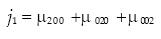
The two–dimensional Cartesian geometric moment (for short 2–D moment) of a 2–D object R is defined as Hu (1962):

...............................................(1)

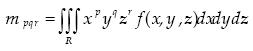
where f(x,y) is the characteristic function describing the intensity of , and p+q is the order of the moment. Similarly, the three–dimensional Cartesian geometric moment (for short 3–D moment) of order p+q+r of a 3–D object is defined as Lo and Don (1989):

......................................(2)

where is a 3–D region. In the case of a discrete binary 3–D image, the moment of a 3–D homogeneous object represented by voxels is often evaluated as:

....................................................(3)

with (x,y,z) ε Z³ and p,q,r =0,1,2,...

2–D moments are important shape features of a 2–D object, and have been widely used in image analysis. Applications of 2–D moments can be found in edge detection (Reeves et al., 1983), texture analysis (Albregtsen et al., 1995), movement estimation (Pei and Liou, 1994), image alignment (Flusser and Suk, 1994), object description (Yang et al., 1995) and object recognition (Dudany et al., 1977) and (Flusser and Suk, 1993). Due to their usefulness lots of efforts have been proposed to reduce the time of computation. Among the most important works we can mention the works of Zakaria et al. (1997), Li y Shen (1991), Jiang and Bunke (1991), Li (1993), Fu et al. (1993), Philips (1993), Yang et al. (1994 and 1996) and Sossa et al. (1999).

The world around us is three–dimensional by nature. 3–D shape information for an object can be obtained by means of computer tomographic reconstruction, passive 3–D sensors, and active range finders. Like the 2–D moments, 3–D moments have been used in 3–D image analysis tasks including movement estimation (Pei and Liou, 1994), shape estimation (Shen and Li, 1993) , and object recognition (Lo and Don, 1989).

The use of 3–D moments is limited due to computational complexity. To compute all moment of order p+q+r < K, a straightforward method needs additions and multiplications of O(K³N³) (assuming that the object is represented by an NxNxN voxel image).

Some fast methods have been proposed to reduce the computational complexity. In Li (1993), Li uses a polyhedral representation of the object for the computing of its 3–D moments. The number of required operations is a function of the number of edges of the surfaces of the polyhedral. The methods of Cyganski et al. (1988), Li and Shen (1992) and Li and Ma (1994) use a voxel representation of the object. The difference among these methods is the way to compute the moments. Cyganski et al.(1988) make use of the filter proposed in Budrikis and Hatamian, 1984). Li and Shen use a transformation based on Pascal triangle for the computation of the monomials; only additions are used for the computation of the moments. On the other hand, Li and Ma (1994) relate 3–D moments with the so–called LT moments that are easier to evaluate. Although these methods allow to reducing the number of operations to compute the moments, they require a computation of O(N³). Recently, Yang et al. (1997) presented a discrete divergence theorem to compute the 3–D moments of an object. It allows a reduction in the number of operations to O(N²). This theorem allows to computing the sum of a function over an n–dimensional discrete region by a summation over the discrete surface enclosing the region.

In this paper we present a method to compute the 3–D moments of a binary region in Z³. The object is first partitioned into convex balls which moment evaluation can be reduced to the computation of very simple formulae instead of using triple integrals. The desired 3–D moments are obtained as the sum of the moments of each ball of the partition, given that the intersection among balls is empty. A first effort in the 2–D case was first presented in Sossa et al. (2001).

The paper is organized as follows. Basic knowledge for better understanding of the paper is given in section 2. The steps of the proposed methodology are deeply explained in section 3. Some experimental results and some final comments are given in Sections 4 and 5.

 

Basic Background

This section presents the basic concepts needed to follow the lecture of the paper. Here the words image and function are used as synonyms; the word volume will be used as synonym of the subset of the image domain. The symbol X will denote an n–dimensional discrete space being a subset of the n–dimensional real space. Most of the times we will work onto a finite subset of (the volume of the integers).

 

Metric and erosions

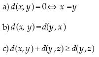
Definition 1. A function d: X R⁺ is called a metric (or distance) iff for all x, y,z ε X, it holds that:

 

Definition 2. The distance function between two points p,q ε X, is defined as

.........................................................(4)

is called ∞ –metric.

 

Definition 3. The pair (X,d), where d is a metric is called a metric space.

 

Definition 4. Given a metric space (X,d), the set defined by:

...........................................................(5)

is called a closed ball of radius t with center in p ε X

 

Definition 5. Let B be a subset of X and p ε X, the translation of B by p is defined as:

............................................................(6)

 

Definition 6. Let A and B subsets of X, the erosion of A by B denoted by A θ B, is defined as:

...........................................................(7)

 

The methodology

Moments of a ball in d_∞ metric

The main idea behind the proposed methodology consist of:

1. Decompose the given shape into a union of disjoint balls; we do this by iteratively eroding the shape of interest by means of the method next described in section method based on iterated erosions to get the partition.

2. Compute the geometric moments for each of these balls, and

3. Obtain the final moments as a sum of the moments computed for each ball

As mentioned before, a first effort in the 2–D case was first presented in Sossa et al. (2001). Clearly, the process involved to compute the moments of the balls will be simpler and cheaper (in time and resources), as the ball structure is simpler. The d_∞ metric has been chosen as it allows us to generate some of the most–simple balls (cubes in a discrete Cartesian plane).

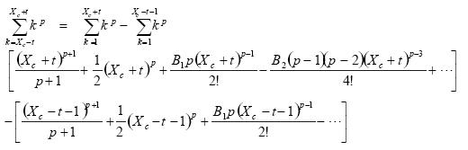
Before continuing we need to derive the set of expressions that will allow us to compute the geometric moments for each cube using the d_∞ metric in terms of their radius and center. To obtain this set of expressions, let us consider a cube centered (X_c,Y_c ,Z_c) with radius t and coordinates of its vertices in

Let us also consider well–known Bernoulli's formulation (Yang and Albregtsen, 1994–1996):

....................................(8)

where the last term of the series contains n or n², depending on if p is even or odd respectively. The Bj's denote Bernoulli's numbers (Yang and Albregtsen, 1994–1996).

The sum of the powers in direction x for a cube R, can be found by means of equation (8). The limits of the summation are: X_c – t and X_c + t, thus:

....(9)

Analogously, for all coordinates in directions y and z, we have that:

......(10)

and

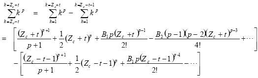...(11)

When applying equations (9) to (11) to equation (8), we obtain the expressions for the moments of order p+q+r for a cube R of radius t centered at (X_c, Y_c,Z_c ). For example, expression for moment m₀₀₀ is:

............(12)

The reaser can easily show that:

 

Method based on iterated erosions to get the partition

The following method to compute the geometric moments of a 3–D object R Z³, using morphological erosions is a direct extension to the one described in Sossa et al. (2001). It is composed of the following steps:

1. Initialize 20 accumulators Ci=0, for i=1,2,...,20, one for each geometric moment.

2. Make A=R and, B= {(±a, ±b, ±c)a, b, c ε {–1,0,1}} is a 3x3x3 pixel neighborhood in Z³.

3. Assign A A θ B iteratively until the next erosion results in (the null set). The number of iterations of the erosion operation before set appears, is the radius t of the maximal cube completely contained in the original region R. The center of this cube is found in set A just before set appears.

4. Select one of the points of A and given that the radius t of the maximal cube is known, we use the formulae derived in the last section to compute the moments of this maximal cube, the resulting values are added to the respective 20 accumulator, Ci, for 1,2,...,20.

5. Eliminate this ball from region R, and assign this new set to R.

6. Repeat steps 2 to 5 with the new until it becomes .

The method just described gives us as a result the true values of the geometric moments of order (p + q + r) < 3, using only erosions and the formulae developed in Section of the moments of a ball in d_∞ metric.

By their nature, the erosions can be done in a massively parallel computer in pretty short processing times. This method is, however, a brute force method (BFM). A considerable enhancement can be obtained if steps 4 and 5 are replaced by:

1. Select those points in A at a distance among them greater than 2t and use the formulae given by Proposition 1, to compute the geometric moments of these maximal cubes, and add these values to the respective accumulators.

2. Eliminate the maximal cubes from region , and assign this new set to.

The enhanced method (EM) consists in processing all maximal cubes of the same radius in just a step, coming back to the iterated erosions until the value of the radio t should be changed. At this point it is very important to verify that the eliminated cubes do not intersect with those just eliminated, because one of the important conditions is that the set of maximal cubes forms a partition of the image. Thus one has to guarantee that these maximal cubes be disjoint sets.

 

Experimental Results

Moment computation

The method introduced in this paper is not designed to work on a conventional computer. Experiments were however done on a 233 MHz PC based system. This way, the processing times are only significant when comparing the method eliminating a cube at the time against the method eliminating at the same time all the non–intersecting maximal cubes at the same step.

Both methods were tested on several hundreds of images. All of them are binary and 101x101x101 pixel sized. These images were obtained by generating at random P touching and overlapping cubes of different sizes inside the 101x101x101 image. At the beginning all the locations of the 101x101x101 cube are zero.

The BFM takes on average, over the whole set of images, 320 seconds to compute all moments of order (p + q + r) < 3. The 320 seconds include the time to compute the partition iteration by iteration. The EM requires only about 80 seconds onto 233 Mhz PC based system to compute the same moments. Again the 80 seconds include the time to get the partition. In both cases most of the time is required to obtain the necessary partitions.

 

Efficiency of the computation

With respect to other methods providing the same results as if equation 3 were used, our method is faster, once the partition is obtained. As you can appreciate its complexity is of . To show this, let us suppose that the image has N rows in all the three directions, and that the object occupies the entire intensity volume, we have thus an object composed of voxels, with t its radio. Table 1 lists the number of operations required to compute the first 20 moments by the straightforward method, by those proposed by Cyganski et al. (1988), Li and Shen (1992), Li and Ma (1994) and ours. The computational complexity of the earlier methods shown in table 1 was taken from Yang et al. (1997).

For a given t, our method requires only 36 multiplications and 8 additions to compute the 20 moments. To get these two numbers we just added the number of multiplications and additions required by each of the 20 moments to be computed. requires, for example, 3 multiplications and 1 addition. m₁₀₀ =m₀₀₀ X_c requires 1 multiplication and no additions because it is supposed that the term (2t +1)³ was already computed.

The careful reader can rapidly see from this table that our method is faster than others, even for a small N. The interested reader can easily verify that for greater values of N our method still requires less time. This is due mainly to the fact that our method uses t instead of N to compute the desired moments.

 

Object Recognition

3–D moments as 2–D moments have been used in object recognition. In many cases those moments are not used in their standard form, this is, directly. They are combined some way to obtain quantities a lit bit changing before set of transformations. We are talking about the so–called invariant moments.

In the bi–dimensional case the well–known Hu moments, invariant to translations, rotations and scale changes were derived and used since 30 years (Hu, 1962). In Flusser and Suk (1993) and in Reiss (1991) arrived to the other set of invariants, but before general transformations (affine transformations). In this section we present a set of experiments to test performance of invariants derived from the set of the formulae proposed in section moments of a ball in metric d_∞.

Several invariants can be derived by means of the Fundamental Theorem of Moment Invariants (FTMI), proposed in Sadjadi and Hall (1980). Two ofthem are:

.........................................................................(13)

...........................................................................(14)

with

........................................................(15)

The µ_pqr are computed as:

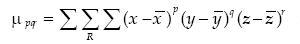............................(15)

with

In this section we show how the invariants moments obtained through the methodology proposed in this paper can be used to differentiate among 3–D objects. In the experiments were used the three objects shown in figure 1: A sphere of radius of 8 voxels, a pyramid with base of 25x25 voxels and a parallelepiped of 55x13x13 voxels. Figure 2 shows three transformed versions (translated, rotated and scaled) of the objects of figure 1. Table 2 shows the values of the corresponding transformations for each object. Table 3 shows the values of the invariant moments for each object's image. In the Table the average times in seconds invested for the computation of the invariants; this includes the time used to obtain the corresponding partitions.

Figure 3, shows the values of the computed invariants for each object (sphere: , pyramid: and parallelepiped: ). From this figure and table 3 the reader can appreciate, in the one hand, that except for class (sphere), the values obtained for the other two classes (pyramid and parallelepiped) change very little inside each class. In the other hand, the differences in the invariants from class to class suggest that any linear classifier could help to differentiate among the three objects used.

 

Conclusions and Future Research

A new method to compute geometric moments for a 3D object has been presented. Initially, the object is partitioned in a set of convex balls whose moment evaluation can be reduced to the computation of very simple formulae. The resulting shape moments are finally obtained by addition of the moments of each ball forming the partition, giving that the intersections are empty. Mathematical Morphology was used to obtain the desired partition of the shape. As the morphological operations implied could be computed in a massively parallel computer, the computation of geometric moments is extremely very fast.

One of the main features of the proposed method is that once the partition is obtained its complexity is of O(N).

Derived invariants derived through the standard moments obtained by the proposed methodology can be also used to differentiate among 3–D objects.

As a future work, we pretend to install this technology to sequential algorithms able to compete with actual algorithms on those computing platforms.

 

Acknowledgments

The authors would like to thank the CIC–IPN, COFAA, CGPI under projects 20050156 and 20060517, and the CONACYT under project 46805 for their economical support to develop this work.

 

References

Albregtsen F., Schulerud H. and Yang L. (1995). Texture Classification of Mouse Liver Cell Nuclei Using Invariant Moments of Consistent Regions, CAIP 95, Proceedings, LNCS 970, pp. 496–502.        [ Links ]

Budrikis Z.L. and Hatamian M.(1984). Moment Calculations by Digital Filters. AT&T Bell Lab. Tech. J. 63:217–229.        [ Links ]

Cyganski D., Kreda S.J. and Orr J.A. (1988). Solving for the General Linear Transformation Relating 3–D Objects from the Minimum Moments, In: SPIE Vol. 1002, pp. 204–211, Bellingham, WA.        [ Links ]

Dudani S.A., Breeding K.J. and Mcghee R.B. (1977). Aircraft Identification by Moment Invariants. IEEE Transactions on Computers, 28(1):39–46.        [ Links ]

Flusser J. and Suk T. (1993). Pattern Recognition by Affine Moment Invariants. Pattern Recognition, 26(1): 167–174.        [ Links ]

Flusser J. and Suk T. (1994). A Moment Based Approach to Registration of Images with Affine Distor tion. IEEE Transactions on Geo–science and remote sensing, 32(2):382–387.        [ Links ]

Flusser J. and Suk T. (1993). Pattern Recognition by Affine Moment Invariants. Pattern Recognition, 26(1): 167–174.        [ Links ]

Fu Ch.W., Yen J.Ch. and Chang Sh. (1993). Calculation of Moment Invariants via Hadamard Transform. Pattern Recognition, 26(2):287–294.        [ Links ]

Hu M.K. (1962). Visual Pattern Recognition by Moment Invariants. IRE Transactions on Information Theory, pp. 179–187.        [ Links ]

Jiang X.Y. and Bunke H. (1991). Simple and Fast Computation of Moments. Pattern Recognition, 24(8):801–806.        [ Links ]

Li B.C. (1993). The Moment Calculation of Polyhedra. Pattern Recognition, 26: 1229–1233.        [ Links ]

Li B.C. and Shen J. (1992). Pascal Triangle–Transform Approach to the Calculation of 3D Moments. CVGIP: Graphical Models and Image Processing, 54:301–307.        [ Links ]

Li B.C. and Ma S.D. (1994). Efficient Computation of 3D Moments, In: Proceedings of 12^th the International Conference on Pattern Recognition, Vol. 1, pp. 22–26.         [ Links ] Lo C.H. and Don H.S. (1989). 3–D Moment Forms, their Construction and Application to Object Identification and Positioning. IEEE Transactions on Pattern Analysis and Machine Intelligence, 11:1053–1064.        [ Links ]

Li B.Ch. and Shen J. (1991). Fast Compu tation of Moment Invariants. Pattern Recognition, 24(8):807–813.        [ Links ]

Li B.Ch. (1993). A New Computation of Geometric Moments. Pattern Recognition, 26(1):109–113.        [ Links ]

Pei S.C. and Liou L.G. (1994). Using Moments to Acquire the Motion Parameters of a Deform able Object Without Correspondences. Image Vision Computing, 12:475–485.        [ Links ]

Philips W. (1993). A New Fast Algorithm for Moment Computation. Pattern Recognition, 26(11):1619–1621.        [ Links ]

Reeves A.P., Akey M.L. and Mitchell O.R. (1983). A Moment Based Two–Dimensional Edge Operator, In: Proceedings of the International Conference on Computer Vision and Pattern Recognition, pp. 312–317.        [ Links ]

Reiss T. (1991). The Revisited Fundamental Theorem of Moment Invariants. IEEE Transactions on Image Analysis and machine Intelligence, 13(8): 830–834.        [ Links ]

Sadjadi F.A. and Hall E. (1980). Three–Dimensional Moment Invariants. IEEE Transactions on Pattern Analysis and Machine Intelligence, Vol. PAMI–2, No 2, 1980.        [ Links ]

Shen J. and Li B.C. (1993). Fast Determination of Center and Radius of Spherical Surface by use of Moments, In: Proceedings of the 8^th Scandinavian Conference on Image Analysis, Tromso, Norway, pp. 565–572.        [ Links ]

Sossa H., Mazaira I. and Ibarra J.M. (1999). An Extension to Philips Algorithm for Moment Calculation. Computación y Sistemas, 3(1):5–16.        [ Links ]

Sossa H., Yáñez C. and Díaz J.L. (2001). Computing Geometric Moments Using Morphological Erosions. Pattern Recognition, 34(2):271–276.        [ Links ]

Yang L., Albregtsen F., Lonnestad T., Grottum P., Iversen J.G., Rotnes J.S. and Rottingen J.A. (1995). Measuring Shape and Motion of White Blood Cells from a Sequence of Fluorescence Microscopy Images, In: Theory and Applications of Image Analysis II (G. Borgefors, Ed), pp. 305–316, World Scientific, Singapore.        [ Links ]

Yang L. and Albregtsen F. (1994). Fast Computation of Invariant Geometric Moments: a New Method Giving Correct Results. Proceedings of the 12th International Conference on Pattern Recognition, Jerusalen, Israel, 201–204.        [ Links ]

Yang L. and Albregtsen F. (1996). Fast and Exact Computation of Cartesian Geometric Moments Using Discrete Green's Theorem. Pattern Recognition, 29(7):1061–1073.        [ Links ]

Yang L. and Albregtsen F. and Taxt T. (1997). Fast Computation of Three–Dimensional Geometric Moments Using a Discrete Divergence Theorem and a Generalization to Higher Dimensions. CGVIP: Graphical models and image processing, 59(2):97–108.        [ Links ]

Zakaria M.F., Vroomen L.J., Zsomrob–Murray P.J.A. and Van–Kessel J.M.H.M. (1987). Fast Algorithm for the Computation of Moment Invariants. Pattern Recognition, 20(6):639–643.        [ Links ]

 

Semblanza de los autores

Juan Humberto Sossa–Azuela. Received his BS degree in Communications and Electronics from the University of Guadalajara in 1980. He obtained his Master degree in Electrical Engineering from CINVESTAV–IPN in 1987 and his PhD in Informa tics form the INPG, France in 1992. He is currently a titular professor of the Pattern Recognition Laboratory of the Center for Computing Research, Mexico since 1996. He has more than 30 publications in international journals with rigorous refereeing and more than 100 works in national and international conferences. His research areas are Pattern Recognition, Image Analysis and Neural Networks.

Francisco Cuevas de la Rosa. Received his BS degree in Compute Sciences from the ITESM, Mexico in 1984. He obtained his Master degree in Computer Science in Artificial Intelligence from the ITESM, Mexico in 1995 and his PhD in Optics Metrology from Centro de Investigaciones en Óptica, A.C., Mexico in 2000. He has more than 20 publications in international journals with rigorous refereeing and more than 40 works in national and international conferences. His research areas are Computer Vision, Optical Metrology, Genetic Algorithms and Neural Networks.

Carlos Aguilar–Ibañez. Received the M. Sc. and Ph. D. In Electrical Engineering from the CINVESTAV–IPN, Mexico in 1994 and 1999, respectively. He is currently a titular professor of the Automatic Control Laboratory of the Center for Computing Research of the, Mexico since 1999. His research interests include nonlinear system, under actuated mechanical system, identification system.

Héctor Benítez–Muñoz. Received his BS degree in Informatics from the Instituto tecnológico de Apizaco, Mexico in 1998. He obtained his Master degree in Computer Science from the Center for Computing Research of the, Mexico in 2005. Actually, he is working at Intermec Technologies of Mexico where he develops wire less applications for mobile systems.