


 nueva página del texto (beta)
 Inglés (pdf)
 Artículo en XML
 Referencias del artículo
 Enviar artículo por email
 Citado por SciELO
  Similares en
SciELO
Similares en
SciELO 
 Permalink
Introduction
Many factors are commonly considered amongst the determinants of well-being, including civil status, household arrangements, and fertility. In this vein, most studies compare married individuals with those who cohabitate, and/or compare those with children to those without children. However, marriage does present some variability, and cohabitation tends to be an even more heterogeneous relationship (Smock, 2000). Hence, researchers should pay closer attention to household arrangements’ diversity (Manning and Smock, 2005).
This paper analyzes associations between different household arrangements for couples and satisfaction with life in Brazil, and it takes into account the natural heterogeneity of marriage and cohabitation. Initially, based on Heuveline and Timberlake (2004) and on Surkyn and Lesthaeghe (2004) as well as on idiosyncrasies of the Brazilian reality, it classified household arrangements of couples into seven different types, one for marriage and six for cohabitation. Thus, the paper proposes a classification for couples’ household arrangements for a developing country, which might be rather different from those observed in industrialized nations.
After this, the paper investigates the relationship between marital arrangements and life satisfaction for couples. Other authors have addressed similar topics in many regions in the world (for instance, Balbo and Arpino, 2016; Blanchflower and Oswald, 2004; Diener, 1984; Dolan et al., 2008; Graham, 2008; Haller and Hadler, 2006; Helliwell, 2006; Perelli-Harris et al., 2019; Slutzer and Frey, 2006), including in Brazil (Corbi and Menezes-Filho, 2006; Gori-Maia, 2013; Islam et al., 2009; Ribeiro, 2015). However, this paper has empirically addressed the natural heterogeneity of both marriage and cohabitation, as the benefits of marriage over cohabitation may depend on personal and household characteristics (Perelli-Harris et al., 2019). Besides, in order to address the endogeneity between household arrangements and satisfaction with life, the link between different household arrangements and different levels of life satisfaction, and also the reverse link, were robustly analyzed using instrumental variables (IV).
Theoretical background
This section presents the background of the paper and describes some of the factors that are commonly considered amongst the determinants of well-being and that are related to household arrangements for couples. For a general discussion of these and other determinants of well-being see Blanchflower and Oswald (2004), Diener (1984), Dolan et al. (2008), and Helliwell (2006).
Marital status is one of the main factors associated with well-being differentials. In general, married people tend to be happier than non-married individuals across different settings and regions (Blanchflower and Oswald, 2004; Diener, 1984; Dolan et al., 2008; Graham, 2008; Gustavson et al., 2016; Haller and Hadler, 2006; Helliwell, 2006; Perelli-Harris et al., 2019; Slutzer and Frey, 2006), and this was also observed with Brazilian data (Corbi and Menezes-Filho, 2006; Ribeiro, 2015). Why are married people happier than others? Married people tend to be wealthier, healthier, and less prone to risky behavior. They also have a “natural” protective net for adverse events in life and a more effective network of help and support. Moreover, marriage is a long-term contract, and may promote a specificity of personal investment, role specialization, and gains of economy of scale (Waite, 1995). Another explanation is due to reverse causality: married people are happier because happier people are more likely to marry and are less prone to divorce (Gustavson et al., 2016; Perelli-Harris et al., 2017, 2019; Slutzer and Frey, 2006).
Nonetheless, many factors may affect marital happiness. VanLaningham et al. (2001) emphasized that most studies observed a U-shaped pattern of marital happiness over the life course. The most widely applied conceptual model for explaining this result focuses on changes in family roles and structures, highlighting the apparent effect of having children in the household. Marital happiness declines as children are added, declines even further as children move into adolescence, and improves as the nest is emptied. Nevertheless, these results may be an artifact of the limitations of cross-sectional data, as period and/or cohort effects may partially explain these results. Indeed, in contrast to this trend, Amato et al. (2003), Umberson et al. (2005), and VanLaningham et al. (2001) observed that marital duration was negatively correlated with marital quality.
Changes commonly associated with the second demographic transition (SDT), which transformed the main features of household formation patterns (Perelli-Harris et al., 2017; Smock, 2000; Surkyn and Lesthaeghe, 2004), are related to period and/or cohort effects. Female labor-force participation increased, creating conflicting demands of work and family for those with small children and thus potentially decreasing marital happiness. The age at first marriage increased, with a postponement of fertility. Cohabitation and divorce rates, and procreation in informal household arrangements, increased. Individual autonomy and expressive values connected to self-actualization became more widespread. Consequently, agreements about gender roles within marriage became less clear, and there was a decline in the prevalence of a traditional family formation sequence in which adults first get married, then live together, and finally have children. (Heuveline and Timberlake, 2004; Perelli-Harris et al., 2017; Treas et al., 2014).
This cultural evolution diminished the earlier disapproval and stigma associated with cohabitation, and cohabitation was free to become widespread (Amato et al., 2003; Perelli-Harris, 2014; Perelli-Harris et al., 2017; Smock, 2000; Treas et al., 2014; Waite, 1995). Normative expectations to marry became feebler, there was a deinstitutionalization-of-marriage, cohabitation acceptance increased in many settings and non-marital arrangements became one among the most prominent behavioral changes affecting family formation (Perelli-Harris et al., 2017, 2019; Treas et al., 2014). Nowadays cohabitation is a common part of the life course of young individuals, and the majority of marriages and remarriages begin with cohabitation (Manning and Smock, 2005; Smock, 2000). Marriage lost its hegemonic position, and boundaries between marriage and non-marital arrangements blurred (Treas et al., 2014).
According to Manning and Smock (2005) and to Perelli-Harris et al. (2019), cohabitation is normally a short experience of a few years, which ends with the termination of the relationship or with marriage. Individuals who cohabitate tend to consider themselves as having a status between singles in a romantic relationship and married individuals. Cohabitators, when compared to married individuals, are less governed by consensual norms and/or formal laws; are less integrated into social support networks; are more oriented toward freedom and independence; and tend to be more individualistic and less committed to the union. However, as cohabitation is a heterogeneous institution and reasons to cohabitate vary across settings (Philips and Sweeney, 2005; Treas et al., 2014), cohabitation might also be viewed as an alternative to marriage -that is, as a long and stable relationship with or without children outside the legal confines of marriage (Perelli-Harris, 2014; Perelli-Harris et al., 2019).
Besides, individuals who cohabitate tend to be different in some other aspects from those who marry. The former tend to have lower socioeconomic status and health levels, and tend to be more liberal, less religious, and more supportive of egalitarian gender roles and nontraditional values than married individuals. Moreover, married individuals show greater family orientation and commitment to their relationships, have more traditional views regarding family roles, and are less prone to ending their relationships than those who cohabitate. In addition, there tend to be fewer differences in age, religion, and race/ethnicity between the partners in married couples than between the partners in cohabiting couples. Finally, children of divorced parents are more likely than others to cohabitate (Dush et al., 2003; Musick and Bumpass, 2012; Perelli-Harris et al., 2019; Smock, 2000).
Probably due to these above-mentioned characteristics, in general, cohabitation does not have the same enhancing effect on well-being as getting married (Perelli-Harris et al., 2019; Smock, 2000). However, non-married couples tend to be as happy as married ones if they perceive that they have a stable relationship (Dolan et al., 2008; Perelli-Harris et al., 2019) and intend to marry (Smock, 2000). Thus, given the heterogeneity verified in marriages and cohabitations, Smock (2000) points out that researchers should pay closer attention to diversity when analyzing civil status, and alternative methods measuring the heterogeneity of cohabitation (and, if possible, marriage) should be implemented (Manning and Smock, 2005; Treas et al., 2014). Dealing with this complexity, Heuveline and Timberlake (2004) proposed six hypothetical types of cohabitation. According to these authors, these types differ in their frequency of incidence, in the proportion of cohabitations ending in marriage, in the duration of the cohabitation, and in the exposure of children to cohabiting parents.
Moreover, parenthood changes the individual´s life in both positive and negative ways (Kohler et al., 2005; Margolis and Myrskyla, 2011). Thus, the relationship Partner + Children = Happiness (Kohler et al., 2005) is not a straightforward one, as having children in the household may increase or decrease well-being levels. Some authors empirically addressed the relationship between parenthood and happiness, and results differ depending on the context and methodology. Some observed positive correlations (Aassve et al., 2012; Slutzer and Frey, 2006), while others verified negative associations (Brown, 2003; Margolis and Myrskyla, 2011; Slutzer and Frey, 2006), or non-significant relationships (Aassve et al., 2012; Peiró, 2006). Besides, results vary depending whether family orientations are more traditional or modern (Balbo and Arpino, 2016).
Regarding parenthood and dealing with the natural heterogeneity of marriage and cohabitation, Surkyn and Lesthaeghe (2004) classified eight types of household arrangements according to non-conformist or conformist values. Married individuals, especially those who had never cohabitated, tended to have a more conventional set of values. Married individuals without children and those who had previously cohabitated were a little less conformist. Conversely, those who were single, those who cohabitated without children, and those who had been formerly in union but at the moment did not have a partner had a more non-conventional set of values. In between were those who cohabitated and had children, and those who still lived in their parents’ households.
Some authors discussed certain particularities of the Brazilian reality concerning the topics under discussion. According to Verona et al. (2015), there are two main characteristics of union patterns in Brazil. First unions are earlier than expected. The strong role of family ties in promoting social and economic stability is one of the main reasons for this trend. Second, the proportion of informal unions has recently grown substantially, in part because informal unions are less expensive than formal marriage. Covre-Sussai (2016) observed they had increased from 6.4 per cent of all unions in 1960 to 36.4 per cent of all unions in 2010, and they were particularly common among lower-income and less-educated couples. Besides, Covre-Sussai (2016) verified that consensual unions in Brazil had a different meaning than in developed countries. Moreover, she also described the striking increase in divorce rates, 500 per cent from 1960 to 2010. Finally, fertility is below replacement level, and rates are still decreasing (Potter et al., 2010).
Based on this theoretical presentation, the first hypothesis of the paper is proposed:
Although in general married individuals might show higher well-being levels than those who cohabitate, some types of consensual union might enhance well-being as much as formal marriage.
The reason is that some individuals who cohabitate may tend to consider themselves as having a status between that of singles in a romantic relationship and that of married individuals, thus they may show lower levels of well-being than married individuals, while others might view cohabitation as a long and stable relationship outside the legal confines of marriage (Manning and Smock, 2005; Philips and Sweeney, 2005) with similar effects on well-being as a formal marriage.
Moreover, taking into account the circular causality between well-being and household arrangements, a second hypothesis is proposed:
Married individuals might have higher levels of well-being because marriage implicates in a more stable relationship that enhances more thoroughly well-being levels than cohabitation, but rather because happier individuals may be more likely to marry and to stay married.
Methods
Data
The Social Dimensions of Inequalities Survey (henceforth SDIS) has as its main objective to evaluate life conditions in Brazil. The survey was conducted in 2008 and contains information associated with demographics, moral values and habits, socioeconomic status, labor market participation, health, and well-being. This database was previously used in studies addressing health issues, class mobility, and education in Brazil (Flor et al., 2014; Laguardia et al., 2011, 2013; Ribeiro, 2014), all with different objectives and approaches than the one applied in this paper.
The survey interviewed 12,423 individuals aged 18 and over, household heads and (when present) spouses, in urban and rural areas of all five Brazilian macroregions with the exception of rural areas of the Northern region. (Only around two per cent of the Brazilian population lives in rural areas in the Northern region. This region is extremely large and heterogeneous.) For this study, only individuals who were married or who lived informally with a significant other were selected. Those who declared that they were single, separated/divorced, or widowed were dropped from the analysis. Moreover, the sample was restricted to those couples who provided information about both individuals. One couple was a homosexual one and it was dropped from the analysis in order to have a more homogeneous sample.
Amato et al. (2003) and Dush et al. (2008) analyzed couples where both spouses were no more than 55 years old. This paper uses a wider range of ages. However, 111 couples had at least one member aged 80 and above, and these couples were dropped from the sample, as it is believed that they might be too aged and might bias the results. The final sample size was 8,288 observations, for 4,144 couples, all with a household head and a spouse in a heterosexual relationship. Household heads and spouses were similarly treated in the empirical analysis.
Household classifications for couples
The SDIS database contains information about individuals who considered themselves as living together or married, irrespective of being legally married. Another variable indicates the nature of the union: if they were united by a civil document and made a religious celebration; if they were united only by a civil document; if they were united only by a religious celebration; or if the union was consensual. In addition, the database records whether the union was the first one or not. Another variable used to define household arrangements was the time spent in the current union.
The database also records whether the women had children, but does not indicate in which union the women had them. Thus, some assumptions were made. Women in higher order relationships possibly had some of their children in their previous relationships. Thus, the information for children was not considered for higher order unions. For women in a first relationship, even though the child might have been born in a previous fortuitous relationship, he/she had possibly lived with the mother in her current relationship, especially when the relationship was short, defined as shorter than ten years, and the children were possibly young. The database has no information about men’s children. For men the assumption is that, for those in their first union in relationships shorter than ten years, the partner´s children lived in the same household as them.
Based on the discussions presented in Heuveline and Timberlake (2004) and in Surkyn and Lesthaeghe (2004), already cited in the previous section, and on idiosyncrasies of the Brazilian reality, a classification for household arrangements for couples in Brazil was proposed, as shown in Table 1.
Table 1 Classification of household arrangements for couples
| Number | Type of household arrangements for couples |
|---|---|
| 1 | Married/Indistinguishable from married |
| 2 | Alternative to marriage I - Consensual marriage/Living together during at least 10 years in a higher-order union |
| 3 | Alternative to marriage II - Consensual marriage/Living together during at least 10 years in a 1st union |
| 4 | Alternative to marriage III - Consensual marriage/Living together for less than 10 years in a higher-order union |
| 5 | Stage to marriage I - Consensual marriage for less than 10 years in a 1st union with children |
| 6 | Stage to marriage II - Living together for less than 10 years in a 1st union with children |
| 7 | Alternative to singlehood or a prelude to marriage - Consensual marriage/Living together for less than 10 years in a 1st union without children |
Source: Own elaboration using Pesquisa Dimensões Sociais da Desigualdade (PDSD).
Well-being variable
The SDIS directly addresses well-being with two variables: one associated with happiness and another with satisfaction with life, as in many other databases (Jorm and Ryan, 2014). In general, the determinants of both are quite similar (Helliwell, Layard and Sachs, 2016) and hence the most common procedure is to use only one of these variables. This procedure is followed in this paper. The happiness variable has fewer categories than the variable for satisfaction with life. This paper considers satisfaction with life, which is a multidimensional construct that addresses cognitive aspects of subjective well-being (Balbo and Arpino, 2016) and has analogous psychometric characteristics as multiple-item scales (Perelli-Harris et al., 2019).
The variable for satisfaction with life had initially ten categories, as in many other databases, where 1 represents the worst possible life and 10 represents the best possible life. The first two categories, indicating the least satisfaction, were not numerous, and the first three categories were aggregated. Thus, the final variable for satisfaction with life ranged from 1 to 8, as described in Table 2.
Table 2 The variable Satisfaction with Life
| Level of satisfaction with life | Description |
|---|---|
| 1 | Least satisfied with life |
| 2 to 7 | Intermediate levels |
| 8 | Most satisfied with life |
Source: Own elaboration using Pesquisa Dimensões Sociais da Desigualdade (PDSD).
Ordered logistic models with the same set of explanatory variables showed very similar results to OLS models. Thus, it was considered that the variable could be treated as continuous.
Explanatory variables
Many factors are commonly considered amongst the determinants of well-being (Blanchflower and Oswald, 2004; Dolan et al., 2008; Graham, 2008; Haller and Hadler, 2006; Helliwell, 2006; Kahneman et al., 2006) and the empirical analysis in this paper selected some of them. Among the individual attributes, the econometric models include as controls age (continuous: years), aged squared (continuous: years squared), race (1 - White 0 - Non-white), and sex (1 -Male, 0 - Female). Among the socially developed characteristics, those included in this paper were: educational attainment (years of formal education: 0 to 3, 4 to 7, 8 to 10, 11, 12 to 14, and 15); Social Economic Status (SES) level (A continuous variable obtained by PCA with variables indicating the presence or not of assets in the household. These assets are, among others: stove, TV, radio, car, computer, microwave oven and washing machine); workload (daily hours: 0 to 3, 4 to 7, 8, More than 8); health levels (1- Very poor health, 2 - Poor health, 3 - Regular health, 4 - Good health and 5 - Very good health); and unemployment status (1 - Unemployed, 0 - Employed). Features associated with attitudes and beliefs towards self/others/life were also included, such as specific religious affiliation (Catholic [1 - Yes, 0 - No] or Pentecostal [1 - Yes, 0 - No]), and frequency of attending worship services (1 - Once a year, 2 - In Religious holidays, 3 - Once a month, 4 - Once a week and 5 - More than once a week). Besides, a dummy variable showing whether or not the individual had close friends (1 - Yes, 0 - No) was incorporated into the models.
Perry-Jenkins and Claxton (2011) emphasized that the effect of parenthood on well-being is better understood if the analysis includes data from both individuals in the couples conjointly. Thus, the partner´s attributes might also impact on the person´s well-being level (Townsend et al., 2001; Gustavson et al., 2016). The models included the following variables for the partner: health levels, unemployment status, workload, and the existence of close friendships.
Besides, differences between partners might also influence well-being levels. The models included as controls the differences in age, religion, union order (first or otherwise), educational level, and race. Finally, the models included controls for urbanity (1- Urban, 0 - Rural) and macroregion of residence (1 - North, 2 - Northeast, 3 - Southeast, 4 - South and 5 - Center-West).
Empirical strategy
The main objective of this paper is to analyze associations between life satisfaction and different types of household arrangements for couples. In order to overcome some of the limitations imposed by endogeneity while using cross-sectional data, the approach exemplified by Figure 1 was used.
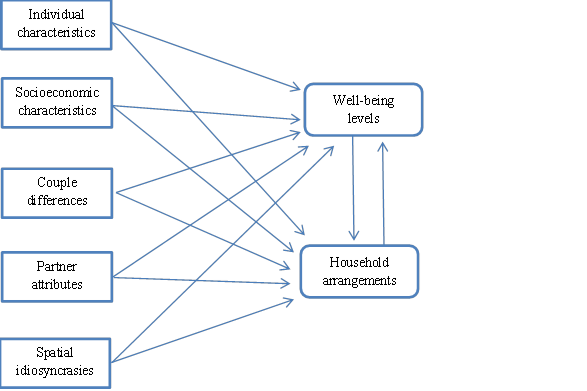
Source: Own elaboration using Pesquisa Dimensões Sociais da Desigualdade (PDSD).
Figure 1 Empirical model of the paper
Individual and socioeconomic characteristics, differences between household head and spouse, partner attributes, and spatial idiosyncrasies, most of which are exogenous variables, influence household arrangements and life satisfaction.
These last two, both endogenous, impact each other (Gustavson et al., 2016): household arrangements influence life satisfaction, and life satisfaction impacts household arrangements.
This model relates life satisfaction to household arrangements, both endogenous variables, and a set of exogenous variables. The following expressions exemplify this association:
(1)y 1 = ƒ(y 2, x i,…, x n), where y 1 is life satisfaction, y 2 is household arrangements, and x i are the n exogenous variables.
(2)y 2 = h(y 1, z i,…, zk), where zj are the k exogenous variables.
The following procedure was proposed for the empirical analysis, which was performed with Stata. First, equation (1) was estimated by standard linear models, remembering that the dependent variable, satisfaction with life, is treated as continuous.
However, the data used in this paper are for couples, and observations are not independent (Hilpert et al., 2016; Kenny and Cook, 1999). Thus, econometric models that ignore the data´s clustering in couples may produce misleading results (Guo, 2005). There are different methods that can be used to overcome this characteristic of dyadic data. Kenny and Cook (1999) presented a review of concepts and proposed different methods. When individuals in the couple are distinguishable, for instance in heterosexual relationships as in this paper, they suggested the use of multilevel modeling. In this approach, individuals are the first level of the model and couples are the second. (For instance, McMahon et al., 2006; Raudenbush et al., 1995; and Townsend et al., 2001). Given that there are only two individuals in a couple, it is often not feasible to estimate random effects for intercepts and slopes simultaneously. Moreover, random slopes may lead to severe convergence problems. Thus, random intercepts may be the best option for multilevel modeling with dyads (Kenny and Cook, 1999; McMahon et al., 2006). Thus, following these advices, a multilevel model was also used to estimate equation (1).
Then the problem of endogeneity was addressed. Following Baum (2006), there are different reasons why endogeneity occurs; simultaneity, as described above, is one of them. Thus, an Ordinary Least Squares (OLS) estimator of either equation (1) or (2) would be biased. A basic procedure is to use instrumental variables (IV), as modeling with Two-stage Least Squares (2SLS); however, the usual 2SLS first stage should be a linear regression (Angrist and Pischke, 2009). If the dependent variable in the first stage is a binary variable and the conditional expectation function is non-linear, as suggested by these authors and used in Adams et al. (2009), a probit model can be estimated, the fitted probabilities computed, and these probabilities used as instrument in the second stage. This was the approach used in this paper. That is, the model with instrumental variable used as dependent variable in the first step a dummy representing whether the union was formal or consensual. Thus, it is a simplification of the many possibilities of consensual unions in order to make the model estimable.
After this, equation (2) was estimated, initially with a multinomial logistic model, as the dependent variable is non-ordered and categorical representing the seven types of household arrangements for couples. Then, a probit regression with a simplification of this equation was estimated with instruments for life satisfaction using the above-mentioned procedure suggested by Angrist and Pischke (2009) and Adams et al. (2009). The dependent variable was a dummy variable (0 - married/indistinguishable from married, 1 - Other informal unions).
Results
Exploratory and descriptive statistics
This section presents exploratory and descriptive statistics of the two variables of main interest of the paper, which are the variable for satisfaction with life and the categorization of household arrangements for couples. Table 3 shows the mean values for satisfaction with life for each type of union. The statistical significances of the comparisons are included in the table. M stands for the larger value and m for the smaller when differences are statistically significant in a particular comparison, which show specific numbers. Comparisons were done with a one-way ANOVA with a Bonferroni ad-hoc test.
Table 3 Mean values for satisfaction with life for different types of household arrangements
| Proposed categorization | ||
|---|---|---|
| 1 - Married/Indistinguishable from married | 5.56 M1 | 0.025 |
| 2 - Alternative to marriage I - Consensual marriage/Living together during at least 10 years in a higher-order union | 5.13 m1,m2 | 0.095 |
| 3 - Alternative to marriage II - Consensual marriage/ Living together during at least 10 years in a 1st union | 5.24 m1 | 0.060 |
| 4 - Alternative to marriage III - Consensual marriage/Living together for less than 10 years in a higher-order union | 5.64 M2 | 0.093 |
| 5 - Stage to marriage I - Consensual marriage for less than 10 years in a 1st union with children | 5.60 | 0.171 |
| 6 - Stage to marriage II - Living together for less than 10 years in a 1st union with children | 5.33 m1 | 0.096 |
| 7 - Alternative to singlehood or a prelude to marriage - Consensual marriage/Living together for less than 10 years in a 1st union without children | 5.40 | 0.143 |
Note: The standard errors were obtained in t-tests.
Source: Own elaboration using Pesquisa Dimensões Sociais da Desigualdade (PDSD).
Notice that married/indistinguishable from married couples (M1) were more satisfied with life than couples whose living arrangements were described as (m1): alternative to marriage I and II or stage to marriage I. Couples whose unions were described as alternative to marriage III, stage to marriage II and alternative to singlehood or prelude to marriage showed non-significant differences when compared to married couples. A second comparison (M2/m2) showed that couples whose unions were classified as alternative to marriage III had significantly higher values for satisfaction with life than couples in the model called alternative to marriage I, and that differences between the former and the other types of arrangements were non-significant. All other possible comparisons were non-significant.
The results suggest that 1 - Married/indistinguishable from married couples showed higher levels of life satisfaction than some informal households, but this was not true for all types of informal households. Arrangements, such as the types (4) and (5), seem to have similar effects on levels of life satisfaction. On the other hand, three arrangements showed lower levels of satisfaction with life: the types (2), (3) and (6). These types of relationships might be viewed as a second-best solution to marriage. Finally, the type (7) shows an intermediate level of life satisfaction
The seven types of household arrangements for couples in Brazil differ in life satisfaction as well as in many other aspects, similarly as observed by Perelli-Harris et al. (2019) and Zimmermann and Easterlin (2006). Table 4 sets out different characteristics of the proposed categories. Married/Indistinguishable from married individuals (1) were the most numerous group among the seven types, representing more than 50 per cent of the total of individuals. (Notice that some numbers are odd, which may seem strange, as the data is for couples. However, household heads and spouses may answer the questions used to classify household arrangements for couples differently). These individuals tended to be in longer-term relationships, and to be older, than those in other types of arrangements. A greater proportion of them were white, and they tended to have lower unemployment rates and higher socioeconomic status. Moreover, they attended religious meetings more often, and a greater proportion of them were Pentecostals and had lived with a father and a mother when they were adolescents. Given these features, and relating these findings with the discussion in Surkyn and Lesthaeghe (2004), possibly they had more conformist views. Health and schooling levels showed intermediate figures, and not higher values as initially expected; this occurred to a great extent because of age, as they are older on average. Notice that individuals in type (1) relationship were most likely to report having a close friend, suggesting a more effective social network.
Table 4 Mean values for different variables for different household arrangements
| Variables | Household arrangement | |||||||
|---|---|---|---|---|---|---|---|---|
| (1) | (2) | (3) | (4) | (5) | (6) | (7) | Total | |
| Number of indivi. | 5,587 | 468 | 1,079 | 452 | 109 | 413 | 180 | 8288 |
| Duration | 22.9 | 20.5 | 20.3 | 7.6 | 8.2 | 7.9 | 6.5 | 20.1 |
| Age | 48.9 | 48.9 | 39.8 | 38.3 | 28.8 | 28.3 | 27.5 | 45.4 |
| White | 52.6 | 41.8 | 35.7 | 43.6 | 47.6 | 37.1 | 45.3 | 48.3 |
| Health | 2.89 | 2.60 | 2.92 | 2.92 | 3.36 | 3.24 | 3.60 | 2.92 |
| Unemployment | 2.29 | 4.08 | 5.34 | 5.11 | 9.42 | 8.67 | 12.51 | 3.57 |
| Income | 1,711 | 992 | 996 | 1,801 | 1,066 | 876 | 1,158 | 1519 |
| Schooling | 7.9 | 6.2 | 7.1 | 7.4 | 9.1 | 8.9 | 10.9 | 7.8 |
| Father/mother | 78.9 | 66.8 | 70.2 | 63.5 | 63.8 | 61.3 | 67.4 | 74.9 |
| Close friendship | 62.0 | 50.8 | 51.0 | 59.2 | 49.4 | 55.1 | 59.1 | 59.2 |
| Catholic | 62.5 | 66.1 | 67.5 | 63.9 | 72.4 | 64.5 | 68.5 | 63.8 |
| Pentecostal | 17.9 | 14.4 | 11.0 | 15.1 | 15.1 | 9.6 | 12.7 | 16.1 |
| Frequency | 3.07 | 2.72 | 2.60 | 2.48 | 2.55 | 2.61 | 2.39 | 2.92 |
Note: (1) Married/Indistinguishable from married; (2) Alternative to marriage I - Consensual marriage/Living together during at least 10 years in a higher-order union; (3) Alternative to marriage II - Consensual marriage/ Living together during at least 10 years in a 1st union; (4) Alternative to marriage III - Consensual marriage/Living together for less than 10 years in a higher-order union; (5) Stage to marriage I - Consensual marriage for less than 10 years in a 1st union with children; (6) Stage to marriage II - Living together for less than 10 years in a 1st union with children; (7) Alternative to singlehood or a prelude to marriage - Consensual marriage/Living together for less than 10 years in a 1st union without children.
Source: Own elaboration using Pesquisa Dimensões Sociais da Desigualdade (PDSD).
Those in relationships classified as (2) or (3) had relationships with similar durations to those of type (1), mostly due to how these groups were defined. That is, they were truly in relationships alternative to marriage, not in short-term relationships ending in breakup or marriage. Those in relationships classified as type (2) had a similar age to those who were classified in in type (1), while those in type (3) relationships were slightly younger. Types (2) and (3) showed smaller proportions of whites and had lower levels of education, lower wages, and higher unemployment rates than married/indistinguishable from married individuals. That is, those in alternative to marriage I and II relationships had a lower socioeconomic status than those who were married/indistinguishable from married. Moreover, the proportion of Catholics was greater, the proportion of Pentecostals was smaller, the frequency of religious attendance was lower, and the proportion who had lived with their fathers and mothers in adolescence was smaller, suggesting that they were less conservative. In addition, the proportion who had close friendships was smaller, indicating a less effective network. Finally, health levels seemed slightly lower when age effects were taken into account.
Those in a relationship classified as type (4) when compared to type (2) were by definition in shorter relationships, and as a consequence were younger. To a great extent, this difference in mean age explains the differences in health, unemployment, and schooling levels. These groups were quite similar in other aspects, such as ethnicity, proportion who had lived with both father and mother as adolescents, and religious affiliation. However, they differed remarkably in income, and in the likelihood of having a close friend, with those in unions described as alternative to marriage III having much higher values.
The types stage to marriage I (5) and II (6) are short-term informal unions where the couples have children. They differ because the couples in type (5) considered that they were married, although not formally, and those in type (6) believed that they lived informally with the significant other, however, in a relationship that could not be subjectively considered a marriage. It was expected that the first would show a greater resemblance to legally married couples, but differences are not great between groups (5) and (6) in most variables. Nonetheless, they differ quite remarkably in three variables. Type (5) shows greater proportions of Whites, Catholics, and Pentecostals. These results suggest that greater proportions of individuals in these three groups of the population consider that, although they are not formally married, their relationships resemble the relationships of those who are legally married.
The comparison between type (7) and types (5) and 6) show some differences besides the existence or absence of children in the household, although all relationships are of short duration and individuals have similar ages. Those in type (7) were healthier, had larger incomes, were more educated, were more likely to have lived with both father and mother as adolescents, had close friendships in greater proportions, and attended religious services less frequently. These results suggest that the group whose living arrangements were described as alternative to singlehood/a prelude to marriage has a higher socioeconomic status and its members will migrate to other types of relationship, selectively choosing formal marriage to a greater extent.
Associations between household arrangements and life satisfaction
This subsection addresses equation (1) with three econometric models. The first model was estimated by OLS (model 1). Given that the data contain couples and observations violate the assumption of independence, a multilevel model (model 2) was estimated with the same set of explanatory variables. In the hierarchical model, couples are the second level. Thus, it is expected that the results of model 2 are superior to model 1, and this last model is included as a benchmark for comparisons. Moreover, given that household arrangements are endogenous, an IV model was estimated (model 3). However, a simplification was made in order to estimate the model and all the non-marriage unions were grouped. Controls were included in the models as described at the bottom of the table, and results are shown only for selected variables.
Some general trends were observed when comparing the three models. Healthy and employed individuals and those who had close friends were more satisfied with life. These findings are not new, and were observed in previously mentioned studies. The individual’s workloads showed mostly non-significant coefficients, suggesting that this is not a main determinant for life satisfaction after controlling for other aspects.
As mentioned, one of the advantages of this study was the possibility of incorporating some variables pertaining to the partner. Individuals whose partners were employed and had higher levels of health were more satisfied with life. The coefficients for the dummy indicating whether the partner had close friends and for the categorical variable for the partner´s workload were non-significant. That is, health levels and employment status of both individuals in the couple were correlated with life satisfaction, whereas for close friendship only the individual´s status seems to matter.
Focusing on variables for union type, only two coefficients were negative and significant in the first model, for relationships types (2) and (6). That is, in a potentially biased analysis only two types of non-marriage unions showed lower levels of well-being than married individuals. However, notice that after controlling for the dependence of the data for couples, in model 2, all coefficients were non-significant. That is, the significant results of model 1 might be caused by biased estimates. That is, model 2 show no difference in well-being levels when the different types of relationships are analyzed. Model 3 showed that when the probability of being in an informal union was addressed with instruments, the coefficient was positive and significant. The result was not at first expected and when compared with the other models, indicates that other factors that affect the propensity of belonging to a formal or informal union, as described in Table 4, might be more relevant to determine the levels of satisfaction with life.
The results in Table 5 indicate that married individuals do not show higher levels of life satisfaction. Similarly, Perelli-Harris et al. (2019) noticed that differences between marriage and cohabitation disappeared when selection and relationship satisfaction were taken into account. The results in this table with a more controlled analysis do not corroborate the findings presented in Table 3, suggesting that other factors controlled in the econometric models are more effective to determine well-being levels.
Table 5 Standard linear, multilevel and IV models addressing the determinants of well-being
| Variables | Model 1- OLS |
Model 2 - Multilevel |
Model 3 - IV |
|---|---|---|---|
| 1 - Married/Indistinguishable from married | Reference | Reference | Reference |
| 2 - Alternative to marriage I - Informal union during at least 10 years in a higher-order union | -0.237** | -0.199 | - |
| (0.0757) | (0.107) | ||
| 3 - Alternative to marriage II - Informal union during at least 10 years in a 1st union | -0.144 | -0.139 | - |
| (0.0756) | (0.0814) | ||
| 4 - Alternative to marriage III - Informal union during less than 10 years in a higher-order union | 0.0141 | 0.00551 | - |
| (0.151) | (0.113) | ||
| 5 - Stage to marriage I - Consensual marriage for less than 10 years in a 1st union with children | -0.0782 | -0.0821 | - |
| (0.238) | (0.203) | ||
| 6 - Stage to marriage II -Living together for less than 10 years in a 1st union with children | -0.289* | -0.230 | - |
| (0.125) | (0.125) | ||
| 7 - Alternative to singlehood or a prelude to marriage - Informal union for less than 10 years in a 1st union without children | -0.243 | -0.234 | - |
| (0.195) | (0.184) | ||
| Informal union | - | - | 0.803* |
| (0.404) | |||
| Very poor health | Reference | Reference | Reference |
| Poor health | 0.665** | 0.668** | 0.676** |
| (0.125) | (0.0994) | (0.102) | |
| Regular health | 0.832** | 0.836** | 0.855** |
| (0.132) | (0.100) | (0.104) | |
| Good health | 1.050*** | 1.050*** | 1.087*** |
| (0.114) | (0.115) | (0.120) | |
| Very good health | 1.290*** | 1.303*** | 1.331*** |
| (0.112) | (0.120) | (0.125) | |
| Partner with very poor health | Reference | Reference | Reference |
| Partner with poor health | 0.101 | 0.0935 | 0.107 |
| (0.146) | (0.0973) | (0.0995) | |
| Partner with regular health | 0.233 | 0.228* | 0.242* |
| (0.143) | (0.0978) | (0.101) | |
| Partner with good health | 0.294 | 0.291** | 0.311** |
| (0.142) | (0.113) | (0.117) | |
| Partner with very good health | 0.403** | 0.381** | 0.423** |
| (0.134) | (0.117) | (0.121) | |
| Unemployed | -0.377* | -0.413** | -0.482** |
| (0.141) | (0.122) | (0.132) | |
| Partner is unemployed | -0.509** | -0.489** | -0.653** |
| (0.178) | (0.121) | (0.138) | |
| Daily workload less than 4 hours | 0.117 | 0.111 | 0.130 |
| (0.0917) | (0.0654) | (0.0676) | |
| Daily workload between 4 and 7 hours | 0.0852 | 0.100 | 0.0903 |
| (0.0749) | (0.0827) | (0.0844) | |
| Daily workload 8 hours | Reference | Reference | Reference |
| Daily workload more than 8 hours | 0.0123 | 0.0162 | -0.00573 |
| (0.0556) | (0.0720) | (0.0739) | |
| Partner´s daily workload less than 4 hours | -0.000912 | 0.0140 | -0.00110 |
| (0.0652) | (0.0634) | (0.0654) | |
| Partner´s daily workload between 4 and 7 hours | 0.00532 | 0.00262 | 0.00236 |
| (0.0865) | (0.0835) | (0.0852) | |
| Partner´s daily workload 8 hours | Reference | Reference | Reference |
| Partner´s daily workload more than 8 hours | -0.0258 | -0.0267 | -0.0327 |
| (0.0943) | (0.0723) | (0.0740) | |
| Close friendship | 0.152* | 0.162** | 0.161** |
| (0.0700) | (0.0481) | (0.0515) | |
| Partner with close friendship | 0.0409 | 0.0457 | 0.0745 |
| (0.0624) | (0.0480) | (0.0532) | |
| Constant | 4.905** | 4.951** | 3.666** |
| (0.591) | (0.413) | (0.619) | |
| Controls for age, race, sex, and place of residence | Yes | Yes | Yes |
| Controls for SES and schooling attainment | Yes | Yes | Yes |
| Controls for religious affiliation and frequency of religious observance | Yes | Yes | Yes |
| Controls for differences between spouses in age, race, religion, and schooling level | Yes | Yes | Yes |
| Observations | 6,323 | 6,323 | 6,323 |
| R-squared | 0.071 | 0.069 | |
| Log likelihood | -12609 |
For OLS models: Robust standard errors in parentheses
For multilevel model: LR test vs. linear regression, prob = 0.0000.
** p < 0.01, * p < 0.05
Source: Own elaboration using Pesquisa Dimensões Sociais da Desigualdade (PDSD).
The association between satisfaction with life and household arrangements
This subsection shows the results of a multinomial logistic model and a probit model with continuous endogenous regressors addressing equation (2): the determinants of household arrangements having satisfaction of life as a explanatory variable. Table 6 shows the coefficients for both models comparing the propensity for belonging to each type of household arrangement when compared to married/indistinguishable from married individuals. Notice that the model with instruments have as dependent variable a dummy which grouped all types of relationship other than married/indistinguishable from married. As is shown in the notes of the table, controls for age, race, and place of residence, and for differences between spouses in age, race, religion and schooling level, were included in the models. However, as they are not the focus of this study, results are not shown.
Table 6 Models analyzing the determinants of household arrangements
| Variables | Model 1 - Multinomial logistic model | Model 2 - Probit model with IV |
|||||
|---|---|---|---|---|---|---|---|
| 2 Alternative to marriage I - Informal union during at least 10 years in a higher- order union |
3 Alternative to marriage II - Informal union during at least 10 years in a 1st union |
4 Alternative to marriage III - Informal union during less than 10 years in a higher-order union |
5 Stage to marriage I - Consensual marriage for less than 10 years in a 1st union with children |
6 Stage to marriage II - Living together for less than 10 years in a 1st union with children |
7 Alternative to singlehood or a prelude to marriage - Informal union for less than 10 years in a 1st union without children |
Informal union | |
| Comparison with: | Married/indistinguishable from married | ||||||
| Satisfaction with life | -0.0708** | -0.0533 | -0.0212 | -0.123** | -0.0603 | -0.145* | -0.293** |
| (0.0199) | (0.0274) | (0.0431) | (0.0308) | (0.0625) | (0.0607) | (0.0398) | |
| SES | -0.0500** | -0.0542** | -0.0778** | -0.0869** | -0.0881* | -0.0330 | -0.0119* |
| (0.0191) | (0.0140) | (0.0100) | (0.0170) | (0.0388) | (0.0287) | (0.00538) | |
| No education | Reference | Reference | Reference | Reference | Reference | Reference | Reference |
| Less than elementary | -0.169 | -0.330* | -0.310* | 0.194 | 0.101 | -0.133 | -0.176** |
| (0.108) | (0.155) | (0.151) | (0.316) | (0.524) | (0.507) | (0.0542) | |
| Elementary | -0.123 | -0.230 | -0.167 | 0.917* | 0.311 | 0.807 | -0.102 |
| (0.176) | (0.144) | (0.216) | (0.374) | (0.520) | (0.452) | (0.0657) | |
| High school | -0.753 | -0.622** | -0.0337 | 0.153 | -0.503 | 1.067** | -0.270* |
| (0.814) | (0.236) | (0.236) | (0.328) | (1.117) | (0.390) | (0.108) | |
| Some tertiary | -0.354** | -0.652** | -0.321 | 0.617 | 0.127 | 1.075* | -0.242** |
| (0.137) | (0.176) | (0.197) | (0.321) | (0.518) | (0.420) | (0.0639) | |
| Catholic | 0.0391 | 0.198 | -0.0268 | 0.0668 | 0.675 | 0.441 | 0.0644 |
| (0.133) | (0.186) | (0.205) | (0.189) | (0.488) | (0.427) | (0.0580) | |
| Pentecostal | -0.149 | -0.436* | -0.0745 | -0.974** | -0.0315 | -0.0628 | -0.118 |
| (0.200) | (0.178) | (0.223) | (0.225) | (0.582) | (0.314) | (0.0675) | |
| Frequency of religious attendance | -0.303** | -0.246** | -0.438** | -0.369** | -0.327** | -0.497** | -0.143** |
| (0.0550) | (0.0492) | (0.0806) | (0.0669) | (0.0879) | (0.0885) | (0.0204) | |
| Lived w. f/m | -0.380** | -0.173 | -0.454** | -0.425** | -0.418* | -0.252 | -0.209** |
| (0.0855) | (0.0926) | (0.0818) | (0.152) | (0.187) | (0.198) | (0.0386) | |
| Partner lived w. f/m | -0.480** | -0.302** | -0.498** | -0.446** | -0.318 | -0.225 | -0.234** |
| (0.103) | (0.0721) | (0.113) | (0.128) | (0.189) | (0.162) | (0.0387) | |
| -3.855** | 0.946 | 1.254 | 7.357** | 1.976 | 8.619** | 3.800** | |
| Constant | (1.031) | (0.582) | (0.836) | (0.886) | (1.461) | (1.465) | (0.225) |
| Observations | 7,430 | 6,323 | |||||
| Pseudo R2 | 0.1862 | ||||||
| Log likelihood | -16069.867 | ||||||
Controls for age, race, and place of residence.
Controls for differences between spouses in age, race, religion, and schooling level.
** p < 0.01, * p < 0.05
For IV model: Wald test of exogeneity, prob = 0.0000
Source: Own elaboration using Pesquisa Dimensões Sociais da Desigualdade (PDSD).
Some general trends are noticed in both models. All coefficients for the Catholic dummy were non-significant. Catholics are still the main group in the Brazilian population and they tend to resemble the whole population of the country (Coutinho and Golgher, 2014). Those with higher level of SES, those who attended religious services more often, those who had lived as adolescents in a household with father and mother, and those who had a spouse who had lived as adolescent in a household with father and mother showed a greater propensity for being married, as coefficients were mostly negative and significant.
These results indicate, as previously mentioned, that cohabitation is particularly popular in Brazil among the lower-income strata of the population. Besides, those who attend religious services with a greater frequency tend to formally marry more often, possibly because they are more conservative. In addition, the experience of adolescent life in the household seems to matter.
More specific results were also noticed. Regarding schooling levels, even controlling for age and income, those with some tertiary education showed a lower propensity for being in alternative to marriage cohabitations for long periods. Moreover, those with higher levels of formal education had a greater propensity for being in unions classified as type (7) relationship. These results suggests that some people in those relationships who have higher levels of formal education may not have children, or may have children afterwards in a relationship classified as married/indistinguishable from married.
Pentecostals showed a smaller propensity for being in a type (3) relationship, indicating a greater conservativeness when in a first union. Besides, they show a lower propensity to be in a short-term informal union with children and consider themselves married.
Concerning the coefficients for satisfaction with life, for the probit model, it was negative, significant and robust, indicating that more satisfied individuals showed a greater propensity to be in a relationship classified as married/indistinguishable from married, suggesting that individuals with higher levels of life satisfaction tend to marry in greater proportion. However, as shown in the multinomial model, the coefficients were all negative, but significant only for three categories. Those who were less satisfied with life were more likely to be in a relationship classified as type (2), (5) or (7), indicating that individuals in these arrangements who had higher levels of satisfaction with life had a greater propensity to marry. Those who had been in informal first unions for at least 10 years, those who had been in informal higher-order unions for less than ten years, and those who had lived together for less than ten years with children showed non-significant coefficients.
The results in this subsection showed that satisfaction with life may influence how individuals choose their household arrangements. Comparing alternative to marriage I and II, the results suggest that those in their first informal union might be a positive selection of those who were initially in a short-term first-order informal union, who might be more likely to end the relationship. A comparison between alternative to marriage I and III suggest that novelty plays a decisive role in higher-order informal unions. The results of stage to marriage I and II indicate that those who considered themselves married and were not formally married were negatively selected in terms of satisfaction with life: a second-best solution. Finally, the results for people whose unions were classed as type (7) indicate that they are also negatively selected when compared to married individuals, as those who are more satisfied with life are more likely to marry.
The results of the last two tables suggest that associations between life satisfaction and household arrangements were significant and robust for equation (2), but not for equation (1). That is, apparently, individuals with higher levels of life satisfaction are more likely to marry or stay married, while the reverse link was mostly non-significant.
Discussion
This paper investigated the associations between marital arrangements and life satisfaction in Brazil. Specific classifications for household arrangements of couples in Brazil were proposed, one for marriage and six for cohabitation. Thus, the paper clarifies some of the limitations of dealing with cohabitation as a single state. In fact, some types of cohabitation resemble singlehood, while others mimic a formal marriage. The implications of these findings for a developing country with high rates of cohabitation can be directly linked with legal practices concerning marriage that should be extended to many couples in cohabitation.
A first hypothesis of the paper was that, although in general married individuals might show higher life satisfaction than those who cohabitate, different types of cohabitation may influence life satisfaction differently, and some types of informal unions might be as life-satisfaction-enhancing as formal marriage. The empirical results corroborated this hypothesis.
Furthermore, this paper emphasizes that household arrangements for couples and well-being cannot be analyzed as a unidirectional relationship, but rather as a potential circular causality (Gustavson et al., 2016). Perelli-Harris et al. (2019) point out that life satisfaction is endogenous to partnership decisions and that happier people may be more likely to marry. They argue that the quality of the relationship may matter more than whether it is legally recognized or not.
Taking into account the potential circular causality between life satisfaction and household arrangements, a second hypothesis was proposed: life satisfaction differentials between household arrangements for couples might be small or nonexistent when it is taken into account that happier individuals may be more likely to marry and to stay married. The empirical results suggest that the link between life satisfaction and some types of household arrangements was significant, whereas that between household arrangements and life satisfaction was non-significant. That is, it seems that married people are more satisfied with their life than people in some other specific household arrangements because individuals who are more satisfied with their life in some arrangements show a greater propensity to marry or to stay married.
A main limitation of the paper is that it uses cross-sectional data. Ideally, the topic should be addressed with longitudinal data (for instance see Gustavson et al., 2016; Perelli-Harris et al., 2019), in which transitions between different types of marriage and cohabitation could be accessed. However, the database used in the paper´s empirical analysis has a great advantage when compared to most others. In general, studies addressing the association of civil status and well-being compare married individuals with those who cohabitate, but do not take into account the natural heterogeneity of both institutions. I could address the natural heterogeneity of cohabitation using the applied database tanking into account those who were married or who lived informally with the significant other, with or without children, and who subjectively considered themselves as married although not legally.

