


 nueva página del texto (beta)
 Inglés (pdf)
 Artículo en XML
 Referencias del artículo
 Enviar artículo por email
 Citado por SciELO
  Similares en
SciELO
Similares en
SciELO 
 Permalink
1 Introduction
The Mexico Basin is home to Mexico City, a megacity with a population exceeding 21 million inhabitants, and accelerated urban growth from the valley towards the mountain slopes. Economic and commercial activities generate high pollution levels, furthering fossil fuel burning due to the demand for mobility [15]. The orographic characteristics of the basin, as it is surrounded by mountains to the east, west, southwest, and south, reduce the ventilation associated with the gap wind system to the southeast and the north [7].
In addition, day-to-day variability in synoptic circulations during the dry season (November to March) can have critical dynamical effects. The synoptic-scale events with a high frequency of occurrence during the dry season are anticyclonic systems that limit dry convection [20], increase stability in the area, giving rise to low-intensity winds, intense radiation, and strong inversions [16].
Under stable conditions, the Mexico Basin has limited ventilation due to the confinement of air masses below the inversion layer, which is limited by the chain of elevated mountains.
This combination of physical processes increases pollutant concentration near the surface in the city and the basin and is the leading cause of health problems for the population at large [25].
In this regard, numerical weather prediction (NWP) by atmospheric models coupled with atmospheric chemistry and aerosol physics modules is crucial for predicting important pollution events within the basin.
The Weather Research and Forecasting System model (WRF) is widely accepted by the scientific community worldwide. The main computational advantage of WRF is that it can be applied to phenomena across broad spatial scales, ranging from tens of meters to thousands of kilometers [26].
The WRF model has been applied to urban problems in the Mexico Basin, with several model configurations that include different physical parametrizations and resolutions.
Jazcilevich et al. [15] use three nested computational domains with resolutions at 27, 9, and 3 km in the configuration of the Penn State/NCAR Mesoscale Model MM5 (the previous generation of WRF) to study flow patterns that affect the concentration of pollutants.
Cui and De Foy [6] apply WRF to study temperature patterns and Urban Heat Island (UHI). López et al. [17] use three nested computational domains at 20, 6.7, and 1 km in a study that analyzes changes in near-surface temperature as they relate to changes in land use land cover change.
Similarly, Ochoa et al. [23] use three domains at 9, 3, and 1 km to analyze changes in precipitation patterns in the basin as they relate to changes in the type of aerosols and land use, land cover changes.
Benson-Lira et al. [3] use four domains at resolutions of 75, 15, 3, and 1 km to evaluate changes in precipitation due to the reduction of Lake Texcoco and the increase of urban area.
The WRF model offers several parametrization schemes for planetary boundary layer (PBL), surface layer parametrizations (SL), and microphysics (MP) schemes, among the most relevant for boundary layer evolution. The PBL and SL schemes are coupled, as the SL provides the lower boundary conditions for the PBL scheme and accounts for feedback between the SL and the PBL schemes.
The WRF PBL parametrizations used in previous studies over the study area are Yonsei University (Y) in ([6, 17, 23]) and Mellor- Yamada-Janjic (M) in ([3]). According to the literature, sensitivity studies abound using different domains and parametrizations for the Mexico Basin.
However, due to the proof-of-concept nature of most of these studies, more attention should be given to the computational performance and the verification against observational data.
To focus mainly on the PBL and the SL schemes, we select a case study in the dry period under weak synoptic forcing and high atmospheric stability.
In this work, we present a series of sensitivity studies that allow the systematic evaluation of: a) spatial resolution, b) boundary layer parametrizations (PBL), surface turbulent fluxes parameters (SL), and c) the microphysics processes involved in cloud formation and vertical motion.
This study provides a way to obtain an optimal configuration particular to the study area in a dry period and under weak synoptic forcing. Therefore, the results of this work are an essential contribution to the air quality forecasting efforts for the Mexico Basin.
The following section details the available data, the technical part of the model, and sets of numerical experiments. In section 3, we present results and discussion. The final section, 4, offers the conclusions and future work.
2 Materials and Methods
2.1 Study Area
Figure 1 shows the terrain features in the Mexico Basin, with almost continuous mountain chains in the west, southwest, and south.
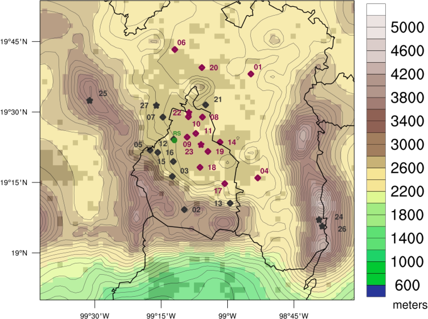
Fig. 1 The topography of the Mexico Basin contours every 100 m. Stations have number tags. Violet and black dots are valley and mountain stations, respectively. Stars and diamonds stations are maintained by the Environmental Monitoring Network of the Ministry of the Environment (SEDEMA) and the National Meteorological Service (SMN), respectively. The green dot represents the radiosonde (RS) launching site position. The black outline indicates Mexico City’s limits within the Mexico Basin. Light gray pixels represent the extent of the current urban area covered by Mexico City and surrounding towns and cities
To the east, mountains are oriented from north to south. In the southeastern of the valley, a gap forms due to the steep descent of the mountainous areas.
The valley is open in the northern part, with small mountain formations in the middle of the valley. The average height of the plateau is about 2200 meters above mean sea level (m amsl). The maximum height of the terrain on the southwest slope is 3930 m amsl.
On the eastern slope, the maximums reach 5400 m amsl due to the Popocatépetl and Iztaccíhuatl volcanoes. The variations in terrain height define the valley in the central part, where the urban area extends mainly towards the slope of the Sierra del Ajusco (see Figure 1).
2.2 Meteorological Data and Case Study
We use surface and radiosonde data to evaluate the performance of the WRF 4.0 model (see Figure 1). Table 1 shows the 28 surface stations, six corresponding to the National Meteorological Service (SMN), 21 stations to the Environmental Monitoring Network administrated by the Ministry of the Environment (SEDEMA), and one station is part of the University Network of Atmospheric Observatories (RUOA).
Table 1 Stations position: ID, Institution (Inst), latitude (Lat), longitude (Lon) and altitude (Alt) of stations
| ID | Inst | Lat(°N) | Lon(°W) | Alt(m amsl) | Name |
| 01 | SEDEMA | 19.64 | 98.91 | 2198 | ACOLMAN |
| 02 | SEDEMA | 19.15 | 99.16 | 2942 | AJUSCO |
| 03 | SEDEMA | 19.27 | 99.21 | 2548 | AJUSCO MEDIO |
| 04 | SEDEMA | 19.27 | 98.89 | 2253 | CHALCO |
| 05 | SEDEMA | 19.37 | 99.29 | 2704 | CUAJIMALPA |
| 06 | SEDEMA | 19.72 | 99.20 | 2263 | CUAUTITLAN |
| 07 | SEDEMA | 19.48 | 99.24 | 2299 | FES ACATLAN |
| 08 | SEDEMA | 19.48 | 99.09 | 2227 | GUSTAVO A. MADERO |
| 09 | SEDEMA | 19.41 | 99.15 | 2234 | HOSPITAL GENERAL |
| 10 | SEDEMA | 19.48 | 99.15 | 2255 | LAB. DE ANALISIS AMBIENTAL |
| 11 | SEDEMA | 19.42 | 99.12 | 2245 | MERCED |
| 12 | SEDEMA | 19.40 | 99.20 | 2327 | MIGUEL HIDALGO |
| 13 | SEDEMA | 19.18 | 98.99 | 2594 | MILPA ALTA |
| 14 | SEDEMA | 19.39 | 99.03 | 2235 | NEXAHUALCOYOTL |
| 15 | SEDEMA | 19.33 | 99.20 | 2326 | PEDREGAL |
| 16 | SEDEMA | 19.36 | 99.26 | 2599 | SANTA FE |
| 17 | SEDEMA | 19.25 | 99.01 | 2297 | TLAHUAC |
| 18 | SEDEMA | 19.30 | 99.10 | 2246 | UAM XOCHIMILCO |
| 19 | SEDEMA | 19.36 | 99.07 | 2221 | UAM IZTAPALAPA |
| 20 | SEDEMA | 19.66 | 99.10 | 2242 | VILLA DE LAS FLORES |
| 21 | SEDEMA | 19.53 | 99.08 | 2160 | XALOSTOC |
| 22 | SMN | 19.50 | 99.15 | 2240 | ENCB II |
| 23 | SMN | 19.39 | 99.10 | 2358 | TEZONTLE |
| 24 | SMN | 19.12 | 98.66 | 4007 | ALTZOMONI |
| 25 | SMN | 19.54 | 99.52 | 3754 | CERRO CATEDRAL |
| 26 | SMN | 19.10 | 98.64 | 3682 | PARQUE IXTA-POPOCATEPETL |
| 27 | SMN | 19.52 | 99.27 | 2364 | PRESA MADIN |
| 28 | RUOA | 19.33 | 99.18 | 2280 | CCA UNAM |
| RS | WYOM | 19.40 | 99.20 | 2313 | Radiosonde SMN |
We classify stations according to altitude. Those with an altitude greater than 2300 m amsl are considered mountain stations, and the rest, regularly located inside the urban area are considered valley stations.
Fourteen stations are located in the mountainous part, while others are on the slopes of the mountains (see Figure 1). In addition, atmospheric vertical profiles are available from radiosondes (RS) launched twice daily at 06 and 18 LST (Local standard time). The launch takes place at the headquarters of the SMN (see Table 1) in the northwest part of Mexico City.
The University of Wyoming gathers radiosonde information around the globe, for Mexico City data can be downloaded from its web page (http://weather.uwyo.edu/upperair/sounding.html accessed on September 4, 2023).
The surface database provides hourly averages for temperature (Tmp), wind direction (Wdr), and wind intensity (Wsp). We use horizontal wind components u (Uhw) and v (Vhw) to avoid spurious results as the statistics for wind direction might be unduly affected by the discontinuity at 0◦-360◦.
Fundamental quality control is applied to the temperature and wind database, eliminating outliers and time series homogenization [2]. The case study is selected from an extensive catalog of daily synoptic patterns for the region using several meteorological criteria: weak synoptic winds, no precipitation, clear skies, high ozone indices, and sufficient data availability.
Analysis of synoptic charts at 500 hPa (≈ 5000 m amsl) and 700 hPa (≈ 3000 m amsl) for February 9-13, 2017, reveals that the study area is under the influence of an anticyclonic system that persists for several days.
Therefore, we select February 10, 2017, as the suitable day, satisfying the above meteorological criteria.
2.3 Weather Research and Forecasting System Model (WRF v4.0)
The Weather Research and Forecasting (WRF) Model is an atmospheric modeling system designed for research and numerical weather prediction.
WRF model is configured to solve the equations of mass, energy, and momentum:
where
The other variables appearing above are the absolute temperature T and the Exner function
The specific heat at constant pressure for dry air is given by
Some major features of the dynamics solver are the following:
– Prognostic Variables: Velocity components u and v in Cartesian coordinate, vertical velocity w, perturbation moist potential temperature, perturbation geopotential, and perturbation dry-air surface pressure.
– Vertical Coordinate: Terrain-following, mass-based, hybrid sigma-pressure vertical coordinate based on dry hydrostatic pressure, with vertical grid stretching permitted. The top of the model is a constant pressure surface. Horizontal Grid: Arakawa C-grid staggering [26].
– Time Integration: Time-split integration using a 2nd- or 3rd-order Runge-Kutta scheme with smaller time-step for acoustic and gravity-wave modes. Variable time step capability [28].
– Spatial Discretization: 2nd- to 6th-order advection options in horizontal and vertical [26].
– Turbulent Mixing and Model Filters: Sub-grid scale turbulence formulation in coordinate and physical space. Divergence damping, external-mode filtering, vertically implicit acoustic step off-centering. Explicit filter option [26].
2.3.1 WRF Computational Details
This study’s experimental design is based on the atmospheric regional model WRF version 4.0 [26]. Initial and boundary conditions of the numerical experiments are obtained from the historical ERA5 global reanalysis [9] produced by the European Center for Medium-Range Prediction (ECMWF), which contains meteorological data on a regular global grid.
ERA5 data are obtained from the Research Data Archive (RDA) repository maintained by the Computational and Information Systems Laboratory at the National Center for Atmospheric Research in the US.
ERA5 reanalysis is available with a spatial resolution of 0.25◦ x 0.25◦ (approximately 30 km x 30 km) beginning in 1979, with hourly time-frequency [9].
WRF code is written in Fortran and C languages and is compiled with Intel(R) Fortran and C compilers version 19 and parallelized using Message Passing Interface (MPI).
Simulations are processed on the Tlaloc supercomputer, housed at the Institute of Atmospheric Sciences and Climate Change and managed by the Computing and High-Performance Unit.
Tlaloc has a 40Gb/s Mellanox® InfiniBand network system that interconnects eleven heterogeneous nodes.
For the numerical experiments in this study, we used only a node featuring four Intel(R) Xeon(R) Gold 6252 CPU @ 2.10GHz with 24 cores in a single thread and 500 GB of RAM.
2.3.2 WRF Parametrizations
As part of the computational design, we select the following physical parametrizations for all simulations: 1) the rapid radiative transfer model for global circulation models [13] simulates the long-wave and short-wave radiation, 2) the Kain-Fritsch scheme simulates shallow and deep convection in the coarsest external domain, while for internal domains the setting is turned off, 3) the Noah land surface model LSM [4] predicts soil moisture, subsurface temperature, hydrology, as well as the interactions between the surface and the atmosphere.
To cover our case study, the experiments start on February 8 at 00 Local Standard Time (LST) (LST=Greenwich Mean Time-6) and end on February 14 at 23 LST, with outputs every hour.
We discard the first 24 hours of the simulation as a part of the model spin-up that allows for the adjustment of the dynamics and thermodynamics of the model. All experiment runs are performed using 36 processors.
WRF binary performs a two-level domain decomposition to parallelize the numerical integration, partitioning the domain in patches (sections of the model domain for each processing node) and tiles (sections of patches to be processed by each core in a node).
To guarantee numerical stability [8], we choose a fixed time step of 2 s for the outermost domain, with a time step ratio of 3 for nested domains.
2.4 Experimental Design
Our approach is first to obtain the best spatial resolution experiment regarding pattern correlation with observational data using Taylor statistics [27] from the six experiments defined below.
Once we obtain the best spatial resolution, we perform a series of sensitivity tests to choose 5 PBL schemes, 5 SL schemes (only those schemes coupled to the PBL schemes), and two microphysics schemes.
2.4.1 Spatial Resolution Sensitivity Experiments SRX
The boundary layer parametrization schemes simulate the diffusion of mass, energy, and momentum by the action of turbulent eddies from the surface to the top of the PBL. They allow its growth by entrainment with the non-turbulent layer above.
SL models, on the other hand, use the theory of Similarity to determine turbulent exchange coefficients of energy, moisture, and momentum fluxes at the surface. These surface fluxes are inputs to the PBL schemes.
We test different computational domain configurations to obtain the optimal spatial resolution, each at a particular spatial resolution.
As such, we propose six experiments where the spatial resolution of the innermost computational domain is set at 1.0, 2.0, and 3.0 km. Three of these experiments use the Mellor-Yamada-Janjic PBL scheme (M), denoted SRX1M, SRX2M, and SRX3M, respectively.
The remaining three experiments use Yonsei University PBL scheme (Y) and are denoted SRX1Y, SRX2Y, and SRX3Y, respectively (see Table 2). All experimental setups use one-way nested grid configurations.
Table 2 Domain configuration and spatial resolution experiment SRX. The distribution of domains is from external to innermost. Ratio refers to downscaling ratios among the domains; the resolution (Res) is the spacing between each point on the mesh, and Dim is the x,y dimensions of the grid in the domain
| SRX | Domains | Ratio | Res (km) |
Dim (x,y) |
| 1 | 1 | 9 | 160,80 | |
| 3.0 | 2 | 3 | 3 | 136,106 |
| 1.0 | 3 | 3 | 1 | 142,145 |
| 1 | 1 | 18 | 99,83 | |
| 2 | 3 | 6 | 81,75 | |
| 2.0 | 3 | 3 | 2 | 63,60 |
Figure 2 shows each computational domain extent, designed to capture orographically forced local phenomena and avoid potential computational instabilities associated with steep mountain regions in proximity to their lateral walls.
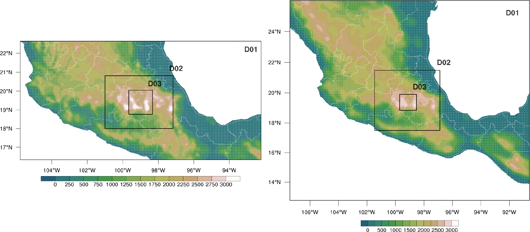
Fig. 2 WRF’s computational domain distribution covering Mexico and the Mexico Basin. The left panel shows the Domains D01, D02, and D03 with horizontal resolution at 9.0, 3.0, and 1.0 km, respectively. The right panel shows the same as the left panel, except for horizontal resolution at 18.0, 6.0, and 2.0 km, respectively. Note that these two domain configurations contain the resolutions of interest for the sensitivity tests, namely, SRX1, SRX2, and SRX3 km
To obtain realistic simulations near the surface and aloft within the planetary boundary layer, all simulations use 76 vertical levels distributed as follows: 20 levels between the surface and 2.25 km, 30 levels between 2.25 km up to a height of 6 km and 26 levels from 6 km to 16 km, the uppermost computational level of the model.
The higher number of computational levels near the surface is required to resolve the turbulent flow fluctuations in mass, energy, and momentum from the atmosphere interaction with the surface.
As mentioned before, we select two PBL schemes that are often used in the literature on mesoscale urban meteorology ([6, 17, 23, 3]) : 1) Yonsei University PBL (Y), and 2) Mellor-Yamada-Janjic (M).
Additionally, both PBL schemes are combined with the Revised Monin-Obukhov Similarity surface scheme and the Monin-Obukhov (Janjic Eta) Similarity surface schemes, respectively. At this stage of the sensitivity testing, we set off the microphysics parametrization (MP) in all of these six experiments.
However, we include the MP scheme to expand the sensitivity testing experiments as explained below.
2.4.2 Boundary Layer (PBL), Surface Layer (SL) and Microphysics (MP) Experiments
Table 3 shows the five selected PBL schemes required to evaluate the sensitivity of WRF’s computational performance to the choice of PBL schemes.
Table 3 Planetary Boundary Layer parametrizations
| PBL scheme option | ID |
| Asymmetric Convective Model | A |
| Mellor-Yamada-Janjic | M |
| Mellor-Yamada Nakanishi and Niino | N |
| Yonsei University | Y |
| Total Energy-Mass Flux | T |
The PBL schemes are the Asymmetric Convective Model version 2 (A) [24], the Mellor-Yamada-Janjic (M) ([18, 19, 14]), Mellor-Yamada Nakanishi and Ninno (N) ([21, 22]), Yonsei University (Y) ([12, 11, 10]), and Total Energy-Mass Flux (T) ([1]).
Table 4 shows the five SL scheme parametrizations used: the Revised Monin-Obukhov Similarity (01), the Monin-Obukhov (Janjic Eta) Similarity (02), the Nakanishi and Niino surface layer (05), the Total Energy -Mass Flux surface layer (10), and the Old MM5 scheme (91). The numbers used match WRF’s manual [26].
Table 4 Surface Layer parametrization
| Land surface scheme | ID |
| Revised Monin-Obukhov Similarity | 01 |
| Monin-Obukhov (Janjic Eta) Similarity | 02 |
| Mellor-Yamada Nakanishi and Niino | 05 |
| Total Energy-Mass Flux surface layer | 10 |
| Total Old MM5 scheme | 91 |
To expand on WRF’s sensitivity to simulation of horizontal wind (i.e, zonal component Uhw, and meridional component Vhw) at 10 meters and upper levels, we proposed experiments with and without MP schemes.
This choice stems from the fact that in the afternoon convective development (which is driven by thermodynamics and microphysics processes) alters local pressure gradients and, therefore, modifies the magnitude of the wind near the surface and aloft. We use the WSM6 as the MP scheme, which is a single-moment parametrization consisting of 6 classes of hydrometeors (see reference for further details [11]).
The MP is used in the higher-resolution nested domains only (i.e., 1.0, 2.0, 3.0, 6.0, and 9.0 km) where convection is resolved explicitly without recourse to a cumulus parametrization. Table 5 shows all 18 experiments, 9 of which have active microphysics with the remaining without it.
Table 5 Sensitivity testing experiments PBL-SL-MP
| No. | MP: ON | No. | MP: OFF |
| 01 | A01n | 10 | A01f |
| 02 | A91n | 11 | A91f |
| 03 | M02n | 12 | M02f |
| 04 | N01n | 13 | N01f |
| 05 | N91n | 14 | N91f |
| 06 | N05n | 15 | N05f |
| 07 | Y01n | 16 | Y01f |
| 08 | Y91n | 17 | Y91f |
| 09 | T01n | 18 | T01f |
The names of the experiments are denoted as follows: the first letter corresponds to the PBL scheme, the following two numbers determine the SL scheme. The activation of the MP is denoted by the final lowercase letter, f (off), to indicate that the microphysics is deactivated and n (on) for the activated option of MP.
Note that the set of experiments is a subset of all possible combinations since not all of them are compatible with each other (see reference WRF’s manual [26]).
2.5 Metrics
In this section, we define a set of metrics that will allow us to find the optimal configuration from all the experiments defined in previous sections. These metrics are based on minimizing simulation errors and execution time.
To obtain the best configuration of physical parametrizations, we use the following four statistical measures: 1) the Pearson’s correlation coefficient (P), the normalized (by the observed standard deviation) root mean square error (RMSE), the ratio of the model standard deviation to that of the observation (SDR), and the bias (B).
where
The
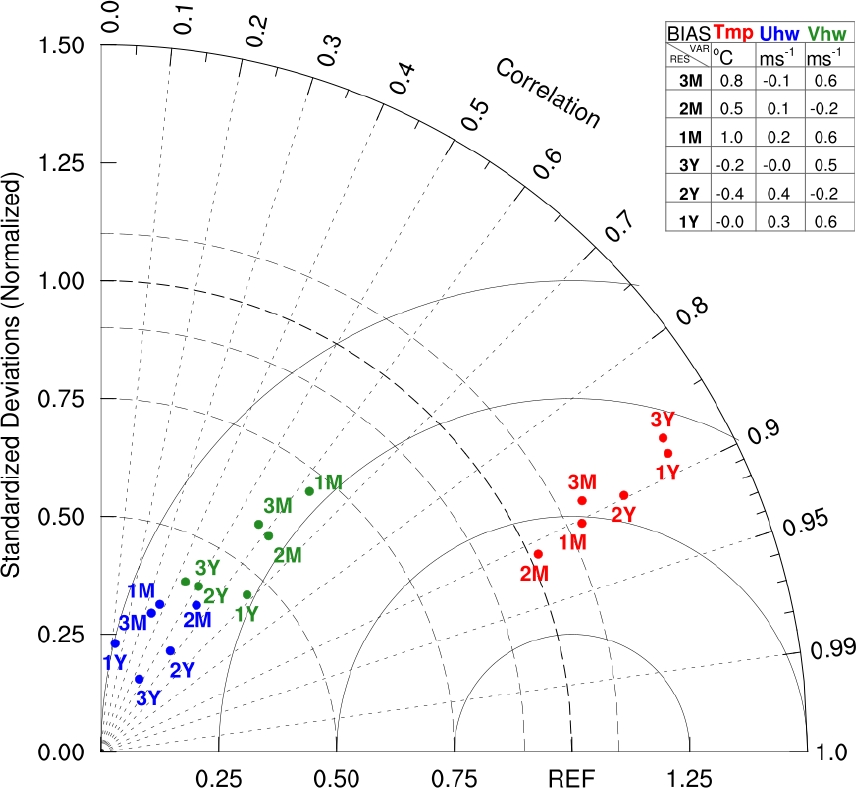
Fig. 3 Taylor diagram for spatial resolution experiments (SRX), tests are performed with M, and Y PBL parametrization. Red, blue, and green labels are for Tmp, Uhw, and Vhw variables. The number refers to resolution, and the letter refers to PBL parametrization. The table shows the bias of each variable
The
The cosine of the angle between the
We only use execution time (ET) as the leading indicator of computational performance since this work focuses on assessing ET’s sensitivity to the selection of physical parametrizations. Therefore, we do not change the number of processors in the proposed experiment suite.
The performance in parallel execution for all experiments is assessed by the ET, which is the time required for the weather forecast application to carry out all the tasks required by WRF to produce a whole simulation run [5].
3 Results
3.1 Sensitivity Study to Spatial Resolution
Figure 3 shows the sensitivity of the SRX experiments using the Taylor diagram with M and Y PBL schemes at 1.0, 2.0, and 3.0 km with their labels as denoted previously.
WRF simulations are evaluated against in situ measurements from surface stations concerning temperature (Tmp).
We find that regardless of spatial resolution, the experiments have a P correlation higher than 0.85 and that simulations overestimate, on average, the observed variability by about 25% (SDR
The correlation coefficient does not decrease significantly, but the M PBL scheme shows closer agreement with observed variability than the Y PBL scheme. For the B metric, we find that SRX1Y shows an almost perfect zero B score while SRX1M shows the most considerable B value of 1.0 ◦C.
Figure 3 also shows WRF’s performance concerning wind components (Uhw and Vhw). WRF simulations underestimate the observed variability by 50% to 80% (SDR
Visual inspection of Figure 3 shows that SRX1M has the best performance for the Vhw component while SRX3Y has the worst. SRX2M shows the best performance, while SRX1Y shows the worst performance.
3.2 Sensitivity Study to Boundary Layer (PBL), Surface Model (LSM) and Microphysics (MP) Selection
3.2.1 Surface Analysis
The previous section has established that WRF’s performance in terms of resolution does not increase continuously as the horizontal resolution is increased.
At this point, we now select the 2.0 km resolution experiments to explore further the sensitivity to include or not the MP scheme, and with three more PBL schemes as detailed in Table 5.
Figure 4 shows Taylor diagrams of variables Tmp at 2m, and Uhw and Vhw at 10 m for the 18 experiments that include the MP scheme (See Table 5). The Tmp variable in the nine experiments with no MP active shows P values higher than 0.89 and lower than 0.91, and all runs overestimate the observed variability. Differences between the experiments are notable in SDR values.
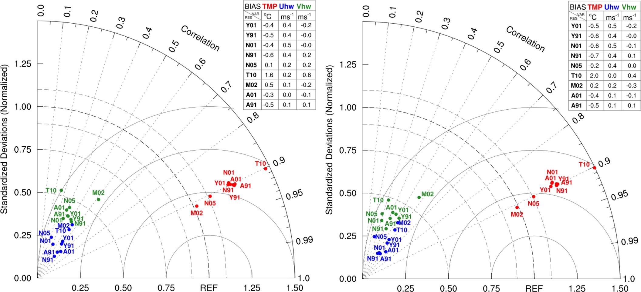
Fig. 4 Taylor diagrams for PBL-LSM-MP sensitivity testing experiments. Red, blue, and green labels are for Tmp, Uhw, and Vhw variables. The first letter refers to PBL parametrization, and the numbers refer to SL schemes. Left and right diagrams show microphysics deactivated and activated, respectively. The table shows the bias of each variable
The M02f run shows values near 1.0, while T10f shows values near 1.5. The remaining nine experiments (right panel in Figure 4) have similar variability. In addition, the T10f run has a more considerable B value at 1.6° C, while the rest of the experiments do not reach 0.7° C.
The Tmp simulation performs better using the M02f at 2 km with SDR near 1.0 and 0.91 Pearson’s correlation value.
Generally, the experiments’ horizontal wind components (Uhw and Vhw) show low P values in the range 0.25-0.7 with SDR values lower than 0.75, and B values do not exceed 0.5
As in the previous section, all experiments with no MP scheme active show WRF’s performance in terms of RMSE, to have lower values in Vhw over those of Uhw (see Figure 4 left panel). The case with MP active is very similar in all metrics to the case with MP set to off (see Figure 4 right panel).
Therefore, in general, RMSE (i.e., distance from the REF point) is very similar for the Uhw and Vhw variables in all cases, with SDR values larger for Vhw than Uhw.
3.2.2 Vertical Analysis
To continue WRF’s performance analysis, we use the vertical profile of Tmp, Uhw, and Vhw from the radiosonde data at 06 and 18 LST. Since values of the Taylor diagram metrics for Tmp are all very close to each other for all experiments, we choose to show the metrics in a table.
Table 6 shows the Taylor metrics P, SDR, and B with MP off and MP on at 06 LST. P values are very close to unity regardless of PBL selection and their coupled SL schemes. SDR values are larger than 0.8 for all nine runs.
Table 6 Taylor metrics for sensitivity testing experiments evaluate with the vertical profile of Tmp (◦C) from the radiosonde data at 06 LST (February 10, 2017). P, SDR and B are the correlation coefficient, standard deviation and bias relative to observations
| EX | P | SDR | B | EX | P | SDR | B |
| Y01f | 0.993 | 0.894 | -5.088 | Y01n | 0.993 | 0.879 | -6.989 |
| Y91f | 0.993 | 0.885 | -6.162 | Y91n | 0.994 | 0.882 | -6.865 |
| N01f | 0.991 | 0.887 | -4.573 | N01n | 0.989 | 0.903 | -1.039 |
| N91f | 0.992 | 0.888 | -5.368 | N91n | 0.990 | 0.901 | -0.468 |
| N05f | 0.990 | 0.885 | -5.151 | N05n | 0.990 | 0.895 | -2.366 |
| T10f | 0.996 | 0.887 | -6.179 | T10n | 0.992 | 0.960 | 7.693 |
| M02f | 0.992 | 0.893 | -4.948 | M02n | 0.996 | 0.881 | -6.939 |
| A01f | 0.992 | 0.889 | -5.293 | A01n | 0.994 | 0.899 | -3.207 |
| A91f | 0.993 | 0.888 | -5.017 | A91n | 0.993 | 0.901 | -4.031 |
However, there are two groups of PBL schemes and their coupled SL schemes that show slight sensitivity of the order of 2-3% to the activation of the MP scheme concerning the runs with MP off: 1) SDR decreases in the Y01n, Y91n, and M02n runs, 2) SDR increases in the N01n, N91n, N05n, T10n, A01n, and A91n runs.
B values indicate the model has a cold bias for observed values except for the T10 experiment, which shows a large shift from -6.18° C with MP off to 7.7° C when MP is on. B values are increased in absolute value for MP off runs for Y01n, Y91n, and M02n runs.
The opposite occurs for N01n, N91n, N05n, A01n, and A91n runs. Therefore, there is a slight sensitivity among the PBL schemes early in the morning, represented by two groups of PBL and their coupled SL schemes responding in an opposite sense to the activation of the MP.
Table 7 shows the same as Table 6 except for 18 LST. At this time, P and SDR values are quite similar among all experiments with MP off and differ very little from the corresponding runs with MP on. On the other hand, B values show improvement with Y01n, M02n, A01n, and A91 but worsen with N91n, N05n, and T10n.
Table 7 Same as Table 6, except for 18 LST
| EX | P | SDR | B | EX | P | SDR | B |
| Y01f | 0.998 | 0.981 | -7.392 | Y01n | 0.999 | 0.981 | -7.158 |
| Y91f | 0.999 | 0.982 | -6.654 | Y91n | 0.999 | 0.986 | -6.657 |
| N01f | 0.999 | 0.978 | -7.297 | N01n | 0.999 | 0.957 | -10.004 |
| N91f | 0.999 | 0.976 | -7.556 | N91n | 0.999 | 0.954 | -10.261 |
| N05f | 0.999 | 0.961 | -6.717 | N05n | 0.998 | 0.967 | -8.585 |
| T10f | 0.997 | 1.052 | 2.670 | T10n | 0.995 | 1.120 | 6.688 |
| M02f | 0.998 | 0.980 | -8.686 | M02n | 0.998 | 0.974 | -7.044 |
| A01f | 0.998 | 0.988 | -7.287 | A01n | 0.999 | 0.984 | -6.262 |
| A91f | 0.999 | 0.984 | -7.144 | A91n | 0.999 | 0.987 | -5.971 |
Figure 5 shows the Taylor diagrams for the Uhw and Vhw wind components at 06 LST (top panels). Inspection of Taylor diagrams with MP off (left panel) and MP on (right panel) reveals contrasting differences between Uhw and Vhw.
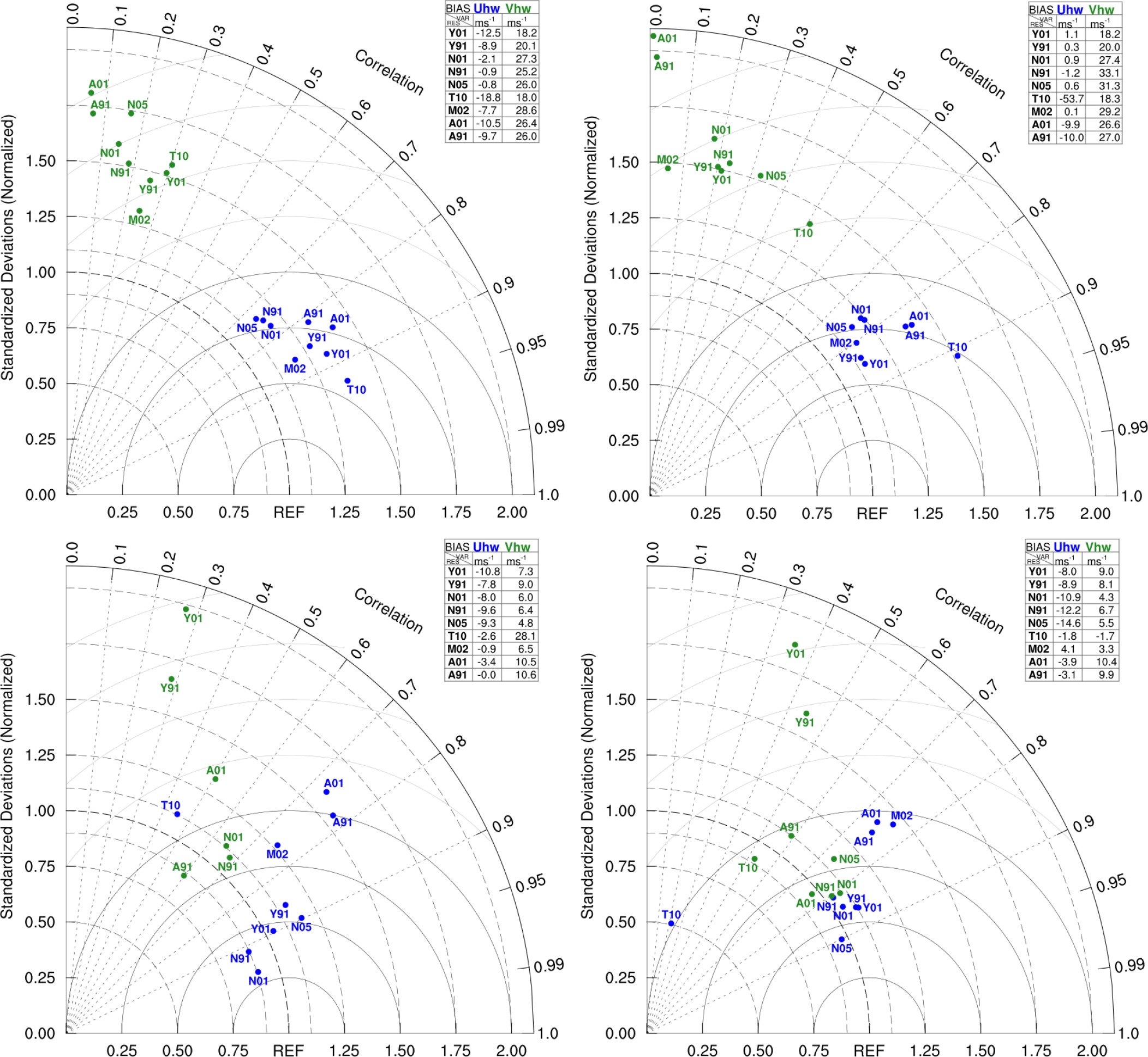
Fig. 5 Taylor diagrams for PBL-LSM-MP sensitivity testing experiments with wind vertical profiles at 06 LST (top panels) and 18 LST (bottom panels). Blue and green labels are for Uhw and Vhw variables. The first letter refers to PBL parametrization, and the numbers refer to SL schemes. Left and right diagrams show microphysics deactivated and activated, respectively. The table shows the bias of each variable
The P values for Uhw range from 0.7 to 0.9
SDR values for Uhw with MP on or off do not vary much and stay around 1.25. B values, however, indicate a strong sensitivity to MP activation.
B values for Uhw varies enormously among PBL schemes from -0.08 up to -12
This pattern distribution of the experiments in the Taylor diagram is not preserved at 18 LST.
Points are more dispersed in the diagram than in the previous diagrams, with some sensitivity to the selection of the MP scheme.
3.3 Computational Performance
Table 8 shows the execution time of the experiments. For a fair comparison among the experiments, we fixed the number of processors to 36 and chose 2 seconds for the time step.
Table 8 Time execution experiments (minutes) with 36 processors
| EX | MPN | MPF |
| Y01 | 77 | 57 |
| Y91 | 76 | 56 |
| N01 | 85 | 65 |
| N91 | 85 | 65 |
| N05 | 85 | 65 |
| T10 | 87 | 67 |
| M02 | 77 | 57 |
| A01 | 82 | 63 |
| A91 | 82 | 62 |
Yonsei University (Y01, Y91) and Mellor-Yamada-Janjic (M02) experiments require less computational time than the rest. The experiments Asymmetric Convective Model (A) and Mellor-Yamada Nakanishi and Niino (N) with their combinations of SL scheme come in second place with approximately 10 more minutes in computational time.
Finally, the experiment with the longest calculation time is Total Energy-Mass Flux (T10). Experiments with the MP scheme on require 20 more minutes of computation time than MP off.
4 Conclusion and Future Work
On the surface, the best performance is obtained by the Mellor-Yamada-Janjic parametrization, which has better performance on Tmp, Uhw, and Vhw. Surface analysis amongst the PBL and their coupled SL schemes with MP on or off shows drastic changes in the metrics of the wind field because MP processes modify the vertical distribution of the flow.
The second best PBL scheme is the Yonsei parametrization, which does a better job in the vertical since it is a parametrization that considers the atmosphere as a whole and thus can better connect low-level convergence with circulation aloft.
WRF’s performance is much better for Tmp than the simulations for wind, which show a higher degree of departure from observations.
Given the complexity of the terrain in the Mexico Basin and the local valley-to-mountain circulations that ensue, the model performance is moderate to represent the wind components.
In this regard, the very different sensitivity to selecting the MP scheme for the horizontal wind components at the surface and its vertical profile is an exciting result.
Wind field simulations close to the observations are a research problem that our group is currently pursuing, and it is part of a more general research program on urban climate that includes a sensitivity analysis of the inversion layer characteristics and temperature profiles that each PBL scheme produces.
Care must be taken when choosing the appropriate parametrization based on the atmospheric processes to be evaluated. In future work, it is necessary to extend the analysis to more case studies under stable meteorological conditions and improve execution efficiency in parallel programming.

