


 nueva página del texto (beta)
 Inglés (pdf)
 Artículo en XML
 Referencias del artículo
 Enviar artículo por email
 Citado por SciELO
  Similares en
SciELO
Similares en
SciELO 
 Permalink
1 Introduction
Surface electromyography (sEMG) signals collected from the contraction movements of the muscles of the upper limbs are a direct representation of the functional status of the muscles. This direct representation has been widely used in medical applications, being the recognition of human motion a significant research topic in the last decades [1].
The potential applications derived from this approach range from developing muscle-computer interfaces (muCIs) [2] to the control of prosthetic devices that makes possible to restore functional capabilities in people who have suffered the loss of a limb [3,4]. Generally, a sEMG automatic signal classification methodology is employed, whereby selected features are extracted from the signals and used to train a classifier algorithm to predict the intended motions of the limbs [5].
The Feature Extraction (FE) technique is a significant step in achieving the optimal performance in classifying the sEMG patterns [6]. Hence, many extraction techniques have been applied to different signal domains, notably in the time domain (TD), the frequency domain (FD), and the time-frequency domain (TFD). Several TD features such as the Mean Absolute Value (MAV), Waveform Length (WL), Root Mean Square (RMS), and Integrated EMG (IEMG) have been effectively used to solve sEMG classification problems [7-9].
However, the TD features are limited to classify small sets of muscle movements [10], since their use requires assuming that signals are stationary so that their statistical parameters are constant in time, though in nature EMG signals are not [5]. The FD features extracted from EMG signals such as the Mean Frequency (MNF), Peak Frequency (PKF), Mean Power (MNP), are not much suitable for classification [10, 11].
Because sEMG signals are not stationary, the recommended approach is often to extract time-frequency (TF) domain features that can be obtained through time-scale analysis methods like Short Time Fourier Transform (STFT) [10, 12], Wavelet Transform (WT) [13] and Wavelet Packet Transform [6]. The WT generate useful subsets of the frequency components of a signal as Wavelet Coefficient Subsets (WCS) [14]. The WT only decompose low frequency components (approximation coefficients) and ignores the effective information in the high-frequency components (detail coefficients) [15].
The WPT allows decomposing the approximation and detail coefficients at the same time based in a binary tree structure [16]. Due to the complexity of the sEMG signals, wavelet coefficients obtained from WT and WPT are widely used as the input features on sEMG classification tasks. Regarding the characterization studies of signals using time-frequency domain methods, several works have shown promising results; for example, Ajitkumar et al. [17] achieve an accuracy of 93.13% for classifying cardiac signals using PCG-ECG.
Specifically, for sEMG signals, Khzeri and Jahed [18] used TD features, STFT, WT and WPT features, and the combination of two domains to classify sEMG signals. Their study showed that the combination of all features (TD + TFD) allowed achieving the best classification results (83%).
However, the influence of choosing WT or WPT features on the classification results was not analyzed, since these were studied together. Subsequently, Phyniomark et al. [19] demonstrated the utility of extracting EMG features (MAV and RMS value) from optimal frequency components (sEMG signals) reconstructed from optimal WCS resulting from WT. The latter, through the comparison of feature extraction from WCS with the characterization of signals reconstructed from the same WCS, showing that the features of the reconstructed signals achieve slightly higher class-separability results than their counterpart.
However, neither a models classification accuracy nor statistical analysis was used to perform a comparison of FE methodologies. In a similar analysis, Shin et al. [16] searched for the best technique to classify EMG signals using four FE methods: TD, Empirical Mode Decomposition (EMD), WT and WPT in conjunction with several dimensionality reduction techniques and classifiers.
They reported that the set of TD features showed the best classification results (over 80%) compared to the other methods. Furthermore, the extraction of WT and WPT features was not performed in the optimal frequency components, as previously suggested, but were extracted from all the wavelet coefficients.
Additionally, a direct comparison between both wavelet methods is not presented. On the other hand, Kevric and Subasi presented a direct comparison between these two wavelet methods [20]; they classified EEG signals by extracting six TD features from the wavelet coefficients obtained from the WT and WPT. They reported that the use of WPT features results in higher accuracy values than the WT features.
This is since the WPT generates a greater number of features than the WT, and because the WPT decomposes the effective high-frequency components of the EEG signals. Subsequently, Xiuwu et al. [15] used the energy and VAR of the WPT coefficients to classify six hand movements with a support vector machine (SVM) achieving an accuracy of 90.66%.
Characterizing the wavelet coefficient vectors with TD features allows eliminating the limitations present when using these features in the time domain [15]. Recently, Bhagwat and Mukherji [5] used the energy of the coefficients from a 4-level WPT as input to a Quadratic Discriminant Analysis (QDA) that reached an accuracy of 99.5% for the classification of fifteen finger movements.
Both WT and WPT have demonstrated excellent performance in classifying upper limb sEMG signals. Nonetheless, we did not find previous work that performed a direct comparison between the time domain feature extraction of wavelet coefficients obtained from WT, WPT and time domain feature extraction for different frequency bands wavelet reconstructed sEMG signals, that allows us to determine which approach is most suitable for hand movement recognition in both performance and computational cost.
The rest of this paper is organized as follows: Section Materials and Methods provides more information about the sEMG dataset being used and describes the signal wavelet decomposition methods, the FE, and the classification. The experimental results and the throughout discussion are presented in Section Results and Discussion. Last section concludes the paper.
2 Materials and Methods
Fig. 1 shows the methodological diagram we followed. The process starts with the EMG raw signals that are conditioned before being processed. After that, there are three pipelines, A) extract TD features from the raw signals, B) from the WCS and C) from the signals reconstructed from the same WCS. The generated features are passed to train the classification models and finally, the models are tested.

Fig. 1 Methodological diagram. The detail (cDn) and approximation (cAn) coefficients generated by the n-level WT and the m coefficients generated by the n-level WPT (cBnm) were characterized or reconstructed for further characterization. Finally, the coefficients and signals were classified
2.1 Database
The sEMG signals were taken from the second sub-database of the 2nd public database generated for the Ninapro Project [21, 23], which is a robust tool that allows comparisons between FE and classification methodologies for sEMG signals in an effort to increase the knowledge in the área of prostheses that function via myoelectric control.
This database contains data recorded from 40 subjects with no degree of amputation (28 males, 12 females, aged 29 ± 3.4 years) while they performed a series of 50 hand movements. Subjects were instructed to imitate the movement displayed on a monitor in front of them.
They performed six repetitions of each movement, each one after a rest period of around three seconds. sEMG signals were acquired through eight electrodes placed around the forearm in relation to the radio-humeral joint, two electrodes were placed at the main points of activity of the flexor and extensor digitorum, and two electrodes were placed on the main activity spots of biceps and triceps muscles.
Fig. 2 depicts a cross-section of the right middle forearm (in palmar supination), specifying the muscles involved in finger and/or wrist movements.
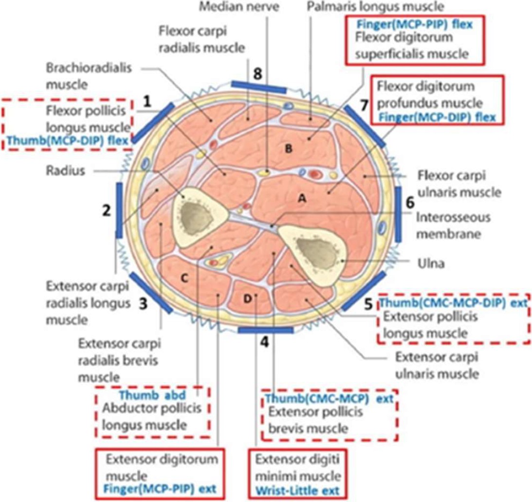
Fig. 2 Cross-section of the right middle forearm. The octagon represents how the electrodes were placed around the forearm. Image retrieved from [24]
The 50 movements (rest included) were divided into four blocks called exercises. Exercise A included information on 12 basic finger movements. Exercise B contained information on 8 hand configurations and 9 wrist movements (see Table 1).
Table 1 Description of the 17 movements in Exercise B
| Movements | No. | Description |
| Hand configurations | 1 | Thumb up |
| 2 | Flexion of ring and little fingers; thumb flexed over middle and little fingers | |
| 3 | Flexion of ring and little fingers | |
| 4 | Thumb opposing base of little finger | |
| 5 | Abduction of the fingers | |
| 6 | Fingers flexed together | |
| 7 | Pointing index | |
| 8 | Fingers closed together | |
| Wrist movements | 1-2 | Wrist supination and pronation (rotation axis through the middle finger) |
| 3-4 | Wrist supination and pronation (rotation axis through the little finger) | |
| 5-6 | Wrist flexion and extension | |
| 7-8 | Wrist radial and ulnar deviation | |
| 9 | Wrist extension with a closed hand |
Exercise C contained information on 23 grasping movements and Exercise D contained information on force patterns which corresponded finger flexion movements. For this work, Exercise B was chosen since it contains hand and wrist movements.
2.2 Experimental Setup
We used the movement and repetition labels from the database to locate each movement and repetition sEMG signal. Movement labels range from 1-18 (rest included) and repetition labels range from 1-6. Subsequently, all EMG channels were normalized to have a mean equal to zero and a unit standard deviation.
Once the signals are normalized, each sEMG signal was decomposed using both wavelet methodologies (WT and WPT), to subsequently extract features from the WCS and from the reconstructed sEMG signals from WCS for further classification.
2.3 Signal Decomposition Using Wavelets
Wavelet transform is useful for processing and analyzing non-stationary biomedical signals. The Discrete Wavelet Transform (DWT) iteratively decomposes a discrete time signal into multi-resolution subsets of signals or wavelet coefficients [19] that represent the frequency components of the input signal, by scaling and shifting a mother wavelet a certain number of times determined by the decomposition level.
At each level, the input signal passes through a high and a low pass digital filter, respectively, and subsequently gets down-sampled by two. The output at each level consists of two signals: approximation (low-frequency components) and detail (high-frequency components) coefficients [20]. For the next level, the approximation signal becomes the input signal, and the process is repeated as many times as levels of decomposition.
Fig. 3A shows a graphical representation of a 6-level WT of a signal sampled at 2kHz. Different features of the input signal can be analyzed from each set of coefficients. One example is the signal trend, which results from analyzing the approximation coefficients associated with the low frequencies of the signal. Other features, such as discontinuities or transient events, can be appreciated by analyzing the detail coefficients, which are related to the high frequencies of the signal [25].

Fig. 3 Graphical representation of wavelet decompositions. A) 6-level wavelet decomposition (WT), the cut-off frequencies of each filter generate the approximation (A) and detail (D) wavelet coefficients. B) 3-level wavelet packet decomposition (WPT)
The WT only decomposes low-frequency components and may miss effective information in the high-frequency components. The Discrete Wavelet Packet Transform (DWPT), moreover, decomposes the approximation signals but also the detail signals at the same time. The detail coefficients also serve as input signals for the next level corresponding to a binary tree structure [15].
DWPT achieves better frequency resolution for the decomposed signal than DWT since, in case of n-levels, DWT generates 𝑛 + 1 frequency components, whereas the number of frequency components produced by the DWPT is the 𝑛-th power of two [20]. Fig. 3B shows the three-level WPT graphical representation for a signal sampled at 2kHz.
Using wavelet decomposition and FE to classify EMG signals have been proposed and used in numerous works [5, 15-19] based on the non-stationarity and complexity of the EMG signals.
In this study, decomposition was performed with both methodologies: WT and WPT.
2.4 Wavelet Decomposition (WT)
For this analysis, a 6-level wavelet decomposition was applied to each channel of the sEMG to divide the signal bandwidth uniformly using the mother wavelet ‘db4’ of the Daubechies family, since it is well known that this mother wavelet is suitable for detecting signal changes and because its shape is similar to the shape of motor units’ action potentials [26, 27]. The decomposition level was chosen trying to match the frequency sub-bands generated by the WT and the WPT.
Since the 3-level WPT generates
Decomposition generated a vector of wavelet coefficients formed by the approximation and the various detail coefficients. Once decomposition was complete, the approximation coefficients corresponding to the level six (cA6) and level 1-6 details (cD1-cD6) were obtained to give seven WCS.
2.5 Wavelet Packet Decomposition (WPT)
In this analysis, the three-level WPT was applied to each channel of the sEMG signals using the mother ‘’db4’’ wavelet. This approach produced a decomposition tree from which we obtained the coefficients corresponding to level three. For each channel of the sEMG signals, we obtained eight WCS (cB31-cB38) that were related to the frequency bands, all with the same resolution (all represented with the same number of coefficients). Table 2 shows the WCS for both WT and WPT and their corresponding frequency sub-bands.
Table 2 WCS generated by a WT and WPT
| 3-level WPT | Frequency Band (Hz) | 6-level WT |
| cB31 | 0-125 | cA6, cD6, cD5, cD4 |
| cB32 | 125-250 | cD3 |
| cB33 | 250-375 | cD2 |
| cB34 | 375-500 | |
| cB35 | 500-625 | cD1 |
| cB36 | 625-750 | |
| cB37 | 750-875 | |
| cB38 | 875-1000 |
Based on the coefficients obtained from both wavelet decomposition methods, the sEMG signals corresponding to each frequency sub-band were reconstructed using the Inverse Wavelet Transform (IWT) [19]. Finally, we characterized the WCS (WDT, WPT) and the sEMG signals reconstructed from their respective WCS.
2.6 Feature Extraction
Once the WCS of the WT and WPT, and the reconstructed sEMG signals were obtained, we characterized them by extracting six TD features from each coefficient vector and reconstructed signal (see Table 3).
The features calculated were mean average value, simple square integral, root mean square value, variance, integrated EMG, and waveform length.
In this way, the dimensionality of each vector and signal was reduced to just a six-element feature vector,
As previously mentioned, converting the WCS or signals into a reduced feature vector represents an important step in classification tasks [20]. Generally, feature extraction can be implemented in two ways. One of them is the feature projection method, which, with the help of artificial intelligence models and dimensionality reduction methods such as Principal Component Analysis (PCA), estimates the best combination of features for the classification task. Here, the characteristics obtained depend on the model used and the dimensionality reduction method [19] and in some cases the features that the model considers are not known [28].
Another method is feature selection and represents less computational complexity [19]; it has been used in many sEMG classification tasks and allows knowing which features are related to the best class separability of upper limb movements.
The EMG feature extraction toolbox provided by Too et al. [29] is used for FE using MATLAB 2017b software (MathWorks).
Finally, we obtained several matrices that stored the information of the movements and repetitions. Each matrix consisted of 108 (18 movements × 6 repetitions) × 73 (12 EMG channels × 6 TD features + 1 label that identified each movement) elements.
2.7 Classification
These matrices were used as input for three classifiers commonly utilized in earlier work on sEMG signal classification: Support Vector Machine (SVM) [5, 15, 16, 30], Multilayer Perceptron (MLP) [16, 33], and Random Forest (RF) [33]. These models are responsible for performing the within-subject supervised multiclass classification of the 18 movements based on their extracted features.
For each subject, out of the total number of features, 80% of the data was used as a training/validation dataset and the accuracy was evaluated using the remaining 20% as the testing dataset.
SVM is a linear classifier that maximizes a mathematical function over a data set [31]. It is designed to maximize classification accuracy while avoiding overfitting the data [32], through the search for the precise hyperplane that segregates the elements of a class from the rest of the classes [33]. We implemented the “one-vs-one” strategy for the multiclass classification.
The MLP is the most widely used type of forward propagating neural network due to its fast operation, easy implementation, and smaller training set requirements [34].
MLP consists of a system of interconnected neurons that represent a nonlinear mapping between the input and output vectors [35]. It is made up of at least three layers: an input layer, one or more hidden layers, and an output layer. Finally, RF is a predictor made up of a set of classifiers structured as trees.
Each tree predicts a classification value for an input value and the class is subsequently decided by the highest voted class value [36].
Hyper-parameters such as the penalty cost (C) of the kernel and its coefficient (γ) of the SVM, the learning rate, the number of neurons in the hidden layer, solver, maximum number of iterations, activation function of the MLP, the estimators number, number of features considered for split, depth of tree and the split criterion of the RF were automatically optimized through the grid-search approach.
This means that for each subject and each frequency component, the hyperparameters of each of the models (SVM, MLP and RF) were optimized.
Evaluations of the three classifiers were performed by stratified leave-one-out cross-validation. This evaluation method was chosen because it allows each folder to hold a proportional distribution of instances that refers to the original dataset. Several metrics are available to evaluate the performance of classifiers.
Accuracy, precisión, and recall are the main measures used for this task [37]. We used the average accuracy value (see Table 4) to report results, defined as the per-class effectiveness of the classifier. The machine learning “scikit-learn” toolbox provided by Pedregosa et al. [39] is used for training and testing of the algorithms using Python 3.9 software.
Table 4 Mathematical definition of the average accuracy value.
| Feature | Definition |
| Average Accuracy [38] |
For an individual
3 Results and Discussion
Results are described in four sections. The first section presents the results of the WCS characterization (WT and WPT). The second shows the results of the classification by the characterization of reconstructed signals from corresponding WCS for both WT and WPT. In the third section, methodologies are assessed; finally, the accuracy of the three models is compared in section four.
3.1 Classification by FE from WT and WPT Coefficients
Fig. 4 shows the average accuracy values obtained by the three classification algorithms when using six-elements feature vectors created by applying Time Domain Feature Extraction (TDFE) to WT-WCS.
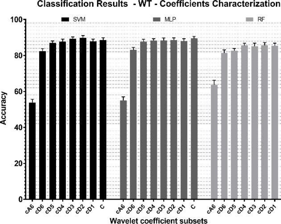
Fig. 4 Classification accuracy when extracting features from the WT-WCS. C represents the result of extracting features from all WCS together, corresponding to the 0-1000 Hz frequency band. The error bars represent the standard error of the mean (SEM)
The best classification results (M = 88.00%) are obtained by the three models in in the WCS cD2 corresponding to 200-500 Hz frequency sub-band (see Table 2). While the lowest classification results (M = 57.54%) are obtained by the three models in the WCS cA6 corresponding to 0-15.6 Hz frequency sub-band (see Table 2).
To evaluate the significance of the changes in accuracy, a series of t-tests were performed, comparing the values obtained for each of the WCS. From these results we observe that the lowest performance results are obtained by the three models in the WCS cA6 corresponding to the 0-15.6Hz frequency sub-band when compared to the rest of the WCS (SVM:
Similarly, the results achieved in the WCS cD6 corresponding to the 15.6-31.2Hz frequency sub-band (M = 82.26%) are significantly lower than those obtained in the other detail bands and those of vector C (SVM:
Consistent with the work of Phyniomark et al. [19] the lowest class separability results are obtained for the WCS cA6 and cD6 corresponding to the 0-31.2Hz frequency sub-band and to the last level of decomposition. However, Phyniomark et al. performed a 4-level decomposition, so they considered the cA4 and cD4 WCS corresponding to the 0-125Hz frequency sub-band as noise. With the 6-level decomposition performed in this work, we can consider the 0-31.2Hz band as noise.
This behavior can be attributed to the lower number of wavelet coefficients
Therefore, we can assume that the optimal WCS to perform the FE are cD5-cD1. Wavelet coefficient vector C achieves similar results but implies a greater number of coefficients than those corresponding to each detail WCS, which translates into a higher computational cost when working with this vector. shows the WCS related to their resolution (number of coefficients).
N is the length of vector C, which is equal to the length of the input sEMG signal. Previous works such as that of Shin et al. [16] achieved accuracy values of less than 80% with a SVM and a MLP, when characterizing the wavelet coefficients of a 4-level WT, in a classification task of 10 hand movements and 20 subjects.
The proposed methodology overcome these results for 18 hand and wrist movements and 40 subjects. Fig. 5 shows the average accuracy values obtained by the three models when using six-elements feature vectors created by applying TDFE to WPT-WCS.
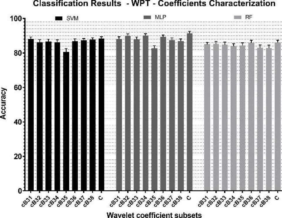
Fig. 5 Classification accuracy when extracting features from the WPT-WCS. C represents the result of extracting features from all wavelet coefficient subsets together, corresponding to the 0-1000Hz frequency band. The error bars represent the standard error of the mean (SEM)
The highest average accuracy values (M = 88.59%, M = 87.29%) for this methodology are observed in wavelet coefficient vector C and in WCS cB36 (625-750 Hz), respectively. While the lowest performance results are observed in the WCS cB35 corresponding to the 500-625Hz frequency sub-band (M = 82.57%).
After statistical analysis, it was observed that WCS cB35 produced significant lower performance results when compared to the rest of the WCS and to wavelet coefficient vector C, by SVM and MLP (SVM:
Previous works have used the characterization of WPT-WCS to solve upper limb movement classification tasks. For example, Shin et al. [16] used the energy of the coefficients of a 4-level WPT in conjunction with an SVM and an MLP and achieved accuracy values greater than 70%.
Both models along with the methodology proposed in this work overcome these results. In an attempt to use the dimensionality reduction of WPT coefficients with TD features, eliminating the drawbacks of using these features on the TD, Xiuwu et al. [15] used the SSI and VAR of the coefficients of a 3-level WPT to classify 6 hand movements of 12 subjects in conjunction with an improved version of the SVM.They achieved an average accuracy of 90.66%.
Our methodology reaches slightly lower values (88.59%) for more movements and subjects; nonetheless, it allows knowing the optimal WCS for FE. Recently Bhagwat and Mukherji [5] achieved an accuracy value of 99.5% when using the log value of the RMS of the coefficients of a 4-level WPT, in conjunction with QDA for the classification of 15 finger movements from eight subjects.
This characterization of all the WPT coefficients implies a higher computational cost than characterizing the optimal sub-bands of the sEMG signals. In future works, we propose the use of the log value of the RMS of the WPT coefficients of the optimal WCS, to see if it is possible to achieve an accuracy value comparable to that achieved by Bhagwat and Mukherji, with a lower computational cost.
From this analysis we can see that similar results were obtained with both methodologies (WT, WPT) when characterizing the coefficients. The principal differences were in the resolution of the WCS (i.e., the number of coefficients considered by each one).
The optimal WCS of the WT to extract features are cD5-cD1, while for the WPT all WCS are optimal except for cB35. It is worth noting that all WCS generated by the 3-level WPT have a resolution of
Table 5 WCS related to their resolution (number ofcoefficients)
| WCS | Resolution |
| C | N |
| cD1 | N/2 |
| cD2 | N/4 |
| cD3 | N/8 |
| cD4 | N/16 |
| cD5 | N/32 |
| cA6, cD6 | N/64 |
Previously, Kevric and Subasi [20] compared both decomposition methodologies –5-level WT and 4-level WPT– when performing a two-class categorization of EEG signals from just 5 subjects. They reported WPT as the best methodology with a classification accuracy of 94.5% compared to WT (81.1%). Their results can be attributed to the fact that the 4-level WPT generated a greater number of WCS (16) than those produced by the 5-level WT (6).
To evaluate the methodologies in approximate equality of conditions (i.e. number of WCS) in this work it was proposed to match the vectors obtained by the wavelet transformations. Seven WCS were obtained for the WT and 8 for the WPT, however, the WT emphasized the low-frequency components, while the WPT emphasized the high-frequency components, losing detail in the low-frequency bands (see Table 2).
We found similar results for both the WT and WPT methodologies (88.00% and 87.29%, respectively). This is by performing multiclass categorization (18 movements) of sEMG signals from 40 subjects.
3.2 Classification by FE of Reconstructed Signals from WT and WPT
Fig. 6 shows the average classification results obtained using the features of the reconstructed signals in different frequency bands from the WT coefficients as inputs to the three classifiers.
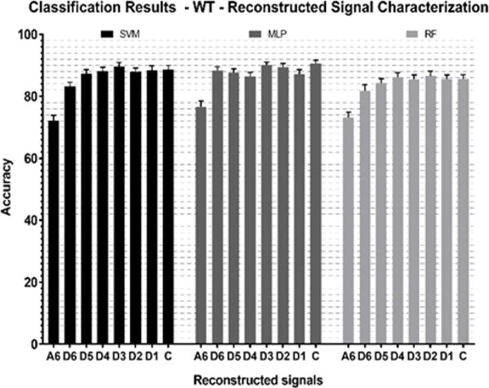
Fig. 6 Classification accuracy when extracting features from the WT reconstructed signals. C represents the result of extracting features from the original sEMG signal (0-1000Hz). The error bars represent the standard error of the mean (SEM)
The highest average accuracy value (M = 88.38%) for this methodology is observed in the reconstructed signal D3 corresponding to the 125-250Hz frequency sub-band. While the lowest accuracy results are observed for the reconstructed signal A6 corresponding to the 0-15.6 Hz frequency sub-band.
As was shown in the previous section, the WCS cA6 produces the lowest accuracy results when classifying. However, when performing the reconstruction of this sEMG signal in the corresponding frequency sub-band associated to this WCS significant higher performance values are reached (M = 57.54%, M = 76.68%, respectively) (SVM:
However, in both methodologies, this frequency sub-band associated to the WCS cA6 can be considered as noise when compared to the rest of the frequency sub-bands.
As in the feature extraction of the WT-WCS, the signal reconstruction from WCS cD6 corresponding to the 15.6-31.2 Hz frequency sub-band reaches lower accuracy values than the rest of the detail bands (M = 84.36%). It was only found that for the MLP the accuracy values of this frequency sub-band are comparable to the rest of the detail bands (SVM:
The average classification results obtained using the features extracted from the reconstructed signals of the WPT coefficients are shown in Fig. 7. The highest average accuracy value (88.02%) is observed for reconstructed signals using the WCS cB35 corresponding to the 500-625Hz frequency sub-band. The lowest average accuracy is observed for reconstructed signals using the WCS cB34 corresponding to the 375-500Hz frequency sub-band (M = 82.98%).

Fig. 7 Classification accuracy when extracting features from the WPT reconstructed signals. C represents the result of extracting features from the original sEMG signal (0-1000Hz). The error bars represent the standard error of the mean (SEM)
Compared with the results of the WCS characterization, the feature extraction of the B35 frequency sub-band reconstructed signal produces significantly better results (82.58%, 88.02%, respectively) (SVM:
This behavior is attributed to the resolution considered by each methodology (FE from coefficients:
Finally, although the lowest results were observed in band frequency sub-band B34, these are not significantly lower than the rest of the sub-bands except for B35 (SVM:
However, the results of the B35 sub-band are significantly better than the results of the rest of the sub-bands (SVM:
3.3 Classification by Coefficient Characterization Vs Reconstructed Signal Characterization
The results obtained using these two methodologies (FE from WCS and FE from reconstructed sEMG signals) are similar. However, as discussed in the previous sections, feature extraction of the reconstructed sEMG signals achieves significantly better results when using the A6 sub-band (WT) and the B35 sub-band (WPT).
This behavior is attributed to the resolution of the sEMG signal
Phyniomark et al. [19] compared both methods and reported slightly superior results when extracting features from the signals. The statistical analysis carried out in this work shows that for the proposed methodology, the differences between the methods are not significant.
These results indicate that both procedures can be used to classify sEMG signals with an average accuracy above 87%. It is important to note, however, that there are differences in resolution between WT and WPT, and that computing costs differ between characterization with WCS and signal reconstruction from those WCS.
On the other hand, we can highlight from signal reconstruction characterization that signal reconstruction is a process equivalent to applying a band-pass filter to the original sEMG signal, so it can be implemented with cutoff frequencies defined in the frequency sub-bands, then after, characterize and classify the signal expecting higher classification percentages similar to both methodologies (D5-D1, B35).
In addition, implementing the filter can be achieved analogically, leaving only the feature extraction and classification processes to the software.
3.4 Classification of sEMG Signals Using SVM, MLP and RF
Based on the classification results, we were able to observe that the results achieved by the RF tend to be lower than those achieved by the SVM and the MLP. Therefore, we decided to compare them statistically in order to determine if this trend is significant statistically.
Table 6 and Table 7 show the p-values of the significant differences found when comparing the accuracy of the models, for the FE from WCS and from the reconstructed signals, respectively.
Table 6 Significant differences when comparing the accuracies of the models when classifying from the FE of the WT-WCS and reconstructed signals
| WCS | Reconstructed Signals | |||||
| SVM vs MLP | SVM vs RF | MLP vs RF | SVM vs MLP | SVM vs RF | MLP vs RF | |
| A6 | 0.00 | 0.00 | ||||
| D6 | 0.00 | 0.00 | ||||
| D5 | 0.01 | 0.00 | ||||
| D4 | ||||||
| D3 | 0.04 | 0.04 | 0.01 | |||
| D2 | 0.03 | |||||
| D1 | ||||||
| C | 0.00 | 0.00 | ||||
Table 7 Significant differences when comparing the accuracies of the models when classifying from the FE of the WPT-WCS and reconstructed signals
| WCS | Reconstructed Signals | |||||
| SVM vs MLP | SVM vs RF | MLP vs RF | SVM vs MLP | SVM vs RF | MLP vs RF | |
| B31 | 0.04 | |||||
| B32 | 0.01 | 0.04 | ||||
| B33 | ||||||
| B34 | 0.02 | 0.00 | ||||
| B35 | ||||||
| B36 | 0.00 | |||||
| B37 | 0.03 | 0.03 | ||||
| B38 | 0.01 | 0.03 | ||||
| C | 0.00 | |||||
When comparing models, A vs B, for example SVM (A) vs. RF (B), a red label shows an increase in accuracy for model B. A green label represents an increase in accuracy for model A.
Consistent with our observations, the statistical analysis shows that both the SVM and the MLP reach higher accuracy values than the RF in several cases. In fact, RF only outperform MLP or SVM when using WT-WCS cA6 features.
We might assume that RF works better with low-frequency features, however, RF does not outperform the other models when using the low-frequency features of the WTP-WCS, which have higher resolution than its counterparts. Therefore, we could assume that RF works better with lower-resolution WCS.
Furthermore, the behavior of the SVM and the MLP are comparable, they even show no difference in their behavior when classifying any of the WT-WCS (see Table 6) or any of the reconstructed WPT-signals (see Table 7). Concerning the significant differences found, the SVM and the MLP perform better than the RF in all cases, except when comparing them in the A6 WCS (see Table 6).
However, even for this model this WCS generates the lowest classification results. When comparing models, A vs B, for example SVM (A) vs. MLP (B), a red label shows an increase in accuracy for model B. A green label represents an increase in accuracy for model A.
The highest average classification accuracy, per model, for the 18 movements are 90.05%, obtained with MLP from the reconstructed signal from the WCS cD3, 89.80% obtained with the SVM from the WCS cD2 and, 86.55% obtained with RF from the reconstructed signal from the WCS cD2.
Also, it can be seen that the results obtained from WCS cD4 (62.5-125Hz) and cD1 (500-1000Hz) and their reconstructed counterparts (D4 and D1) are independent of the classification model, this behavior can also be observed for the WCS cB33 (250-375Hz) and cB35 (500-625Hz). This could be attributed to the fact that the features obtained from these WCS, and reconstructed signals are sufficiently robust to achieve comparable results for all three models.
Consistent with the work of Shin et al. [16] who used the SVM and the MLP to classify 10 hand movements, both models reach the highest results compared to other models, in the case of Shin et al. QDA, K-Nearest Neighbor (KNN), and Extreme Learning Machine (ELM).
4 Conclusions
This paper presents a comparison of various sEMG signal characterization methodologies. We observed that WT characterization obtain comparable results as WPT using WCS with small number of coefficients. When extracting characteristics of the WT-WCS, the optimal subsets are cD5 to cD1 corresponding to the 31.2-1kHz frequency sub-band, however, the WCS cD5 is the one with the lowest resolution
When using WPT and therefore having more resolution available
Finally, WCS cB35 (500-625Hz), which achieves the worst performance results with a resolution of
Findings also demonstrate that it is possible to characterize sEMG signals at low and high frequencies and obtain similar results when they are classified, which enables the use of systems with low sampling frequency that conserve useful information behind the sEMG activity.
As future directions, we intend to use features, which are known to achieve high accuracy values when classifying sEMG signals, in optimal frequency components in order to know if it is possible to achieve these same values using filtered sEMG signals or low-resolution WCS.
Finally, our results seek to contribute to the knowledge of characterization methodologies and, consequently, to the development of upper limb support technologies.

