


 nova página do texto(beta)
 Inglês (pdf)
 Artigo em XML
 Referências do artigo
 Enviar este artigo por email
 Citado por SciELO
  Similares em
SciELO
Similares em
SciELO 
 Permalink
1 Introduction
Bacterial Vaginosis (BV) is an imbalance of the vaginal flora characterized by the decrease in Lactobacillus before excessive anaerobic bacterial growth [17].
The main affected by BV are women of reproductive age. BV manifests itself clinically as symptomatic or asymptomatic. Symptomatic cases present clinical signs in the genital tract such as vaginal odor, itching, increased vaginal discharge, and pH greater than 4.5 [6].
An early diagnosis of symptomatic cases avoids the development of gynecological complications such as endometritis, salpingitis, oophoritis, pelvic inflammatory disease and susceptibility to acquiring sexually transmitted diseases [4].
BV diagnosis is performed by standardized methods such as the Amsel criteria, the Nugent score, and real-time PCR (Polymerase Chain Reaction). These methods are used especially in epidemiological, clinical and microbiological investigations to study, understand and document the normal and anaerobic flora involved in the development of this condition.
However, BV is a complex issue due to the large vaginal microbiological ecosystems, with a pathogenesis that is still unclear [21]. Especially, we know that a BV-positive condition is a dysbiosis between the microorganisms existing in the vaginal mucosa.
However, the coexisting bacteria may differ from patient to patient, and individual analysis does not make it possible to identify contexts between patients. So it is of our interest to tackle this problem using a partitional clustering approach.
Our purpose is to provide a clustering model of patients that allows a detailed analysis of the coexistence of bacteria in groups with a common diagnosis.
In the current literature, few studies have been conducted using Machine Learning (ML) to build computational models that support understanding a complex condition such as BV.
For example, the study performed by Song et al. [22] integrated superpixel methods with Deep Learning methods based on a Convolutional Neural Network (CNN) for the automatic assisted diagnosis of BV.
Another study was conducted by Baker et al. [2] in which a classification model was constructed by breaking down the microbial groups according to their correlation. In the research of Pérez-Gómez, J. F et al. [16] determined the most relevant predictor attributes of BV in a dataset using five attribute selection algorithms.
2 Materials and Methods
2.1 Dataset
In this study used a dataset of BV bacteria from samples collected from women aged 18 to 50 in urban populations in Comalcalco, Tabasco, Mexico.
The microorganisms comprising the dataset were obtained by semiquantitative PCR at the Infectious and Metabolic Diseases Research Laboratory of the Juárez Autonomous University of Tabasco as part of BV research in molecular epidemiology [8].
This dataset is complete without missing values and was constructed by a biology expert. The dataset consists of 201 patient records with 15 attributes corresponding to microorganisms implicated in BV, see Table 1.
Table 1 Attributes corresponding to BV microorganisms used in our study which were introduced in [19]
| Attribute | Description |
| CrispatusCq | Lactobacillus Crispatus Cq* Growth Value |
| InersCq | Lactobacillus Iners Cq* Growth Value |
| JenseniiCq | Lactobacillus Jensenii Cq* Growth Value |
| GasseriCq | Lactobacillus Gasseri Cq* Groth Value |
| PathogenCom | Pathogen Combination |
| Megasphaera Phylotipo1 | Gram Negative Anaerobic Bacteriam, 16s RNA Sequence |
| Atopobium | Atopobium |
| Gardnerella V. | Gardnerella Vaginallis |
| CT | Chlamydia trachomatis |
| NG | Neisseria Gonorrhoeae |
| HSV1&2 | Herpes Simplex type 1 and 2 |
| MH | Mycoplasma Hominis |
| MG | Mycoplasma Genitalium |
| UP | Ureaplasma Parvum |
| UU | Ureaplasma Urealyticum |
2.2 K-Means Algorithm
The K-Means clustering algorithm is an unsupervised learning partitioning method in ML widely used in the literature. K-Means aims to segment datasets into
A fundamental issue in K-Means is the determination of the optimal number of cluster (
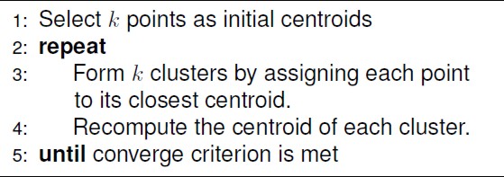
The K-Means algorithm consists of the following steps [1], see Table 1. There are variants of K-Means clustering algorithm, with differences in the criteria for constructing the underlying clusters.
The following criteria are described in the scientific literature: Lloyd [14] considers the distribution of the data to be discrete, Forgy [7] considers the distribution to be continuous, MacQueen [15] considers that the centroids are recalculated every time an observation moves to another cluster and also after each pass through all observations and Hartigan-Wong [8] identifies the data space partition with locally optimal within-cluster Sum of Squares of Errors (SSE).
2.3 Distance Metrics
The distance metrics used to estimate the distance matrices required by a clustering algorithm are described here.
– Euclidean distance. Measures the straight-line proximity between a pair of objects in a n-dimensional space [3]. It is written mathematically as shown in Equation 1:
where
– Asymmetric binary similarity measure. Calculates the proximity between objects with asymmetric binary properties. An asymmetric attribute is a type of nominal variable that has two levels (1-Presence, 0-Absence); this means that one of the two states of the attribute is more informative than the other.
This property is exemplified when we seek to identify the presence or absence of a disease according to its characteristics. Faith, D. P. (1983) [5] suggests the following measure of similarity S, as shown in Equation 2:
where
– Canberra distance. Estimates the distance (
This metric calculates the sum of series of a fraction of the difference between coordinates of a group of objects. Values with zero numerators and denominators are omitted in the sum and are considered non-existent. The formula is defined as shown in Equation 4:
2.4 Metrics for Determining the Optimal Number of Groups
The metrics for determining the optimal number of groups are described in this subsection.
– Gap Statistic. Compares the total intragroup variation for different
where
– Silhouette. Calculates the mean of the observations for different values of
where
– Elbow method. Determines the optimal number of clusters in a data set. This method allows us to explain and verify the consistency of a clustering analysis [13]. It is written mathematically as shown in Equation 7:
2.5 Purity Validation Metrics
Purity is a validation metric that evaluates the quality of a clustering model’s underlying clusters. The purity of the clusters is measured in relation to the class labels, with values ranging from 0 to 1. A value close to 0 denotes poor clustering. A value close to one indicates that the clustering is good [20]. It is written mathematically as shown in Equation 8:
where N is the number of objects,
3 Experimental Design
The present study aims to create a clustering model in which the underlying groups share a common diagnosis to perform a detailed analysis of bacterial coexistence contexts. The partition clustering model was built following the steps, as shown in Figure 1.
– Evaluation of the metrics to determine the optimal number of clusters. The exploration of the different K-Means variants begins with the evaluation of the methods that allow to determine the optimal number of groups, which are the gap statistic, the silhouette and the elbow method.
For the gap statistic and silhouette, the optimal value of clusters is determined when the highest value is reached in the graph.
Whereas for the elbow method, it is determined by observing the graph a decrease from a
– Estimate of the distance matrix of the dataset for each selected distance metric, which are Euclidean, Binary, Canberra. To perform the estimation, the dist function of the stats package was used.
– Model construction using the distance matrices calculated in step 2; each matrix was evaluated using the four K-Means variants.
– Validation of the underlying groups internally and externally. The internal validation of each cluster was determined by estimating the purity percentage described in subsection 2.5. The external validation process, the class label was used, which was hidden from the algorithm to let it do its work.
This process was performed by building a cluster table is a cross-frequency table between the real class variables and the group variable assigned by the algorithm. The column and row structures show the grouping of elements according to the group and diagnosis assigned by the algorithm.
– Comparison of the purity results of each cluster to identify the best grouping. Subsequently, the grouping tables obtained in the step 4 were analyzed to identify, which clusters have been constructed with respect to their actual diagnostic class.
– Biological validation involves verifying the biological significance of the underlying groups in the clustering models. For this purpose, the clusters were made available to an expert in the field.
The expert examined each element of the underlying clusters and confirmed that they were all placed in the correct cluster based on the real class of the elements.
– Use of a data visualization tool to explore the coexistence of bacteria in the groups underlying the best model.

4 Results
To the best of our knowledge, at the time of this study, no other research has been found in the literature that addresses the problem of BV to identifying coexisting bacteria in groups of patients, using machine learning algorithms specifically with a partitional clustering approach.
In this section, we showed the results obtained by applying K-Means variants. The results of the evaluation of the metrics for determining the optimal number of clusters in the dataset were as follows: the gap statistic method, the silhouette method, and the elbow method delivered a value of
Based on the results, it was determined that the
The purity and clustering tables of the models that obtain a positive clustering of patients either in a single group or in different groups are detailed. Each table shows the combination of K-Means variants and a distance measure.
The results allow to evaluate the clustering quality using the purity percentage and the cross-frequency tables. To determine that an underlying cluster has a good object clustering quality, it was considered that the purity percentage was greater than or equal to 0.90.
Furthermore, it is of interest for the study to identify clusters consisting only of BV-positive elements, i.e. all resultant clusters will hold BV-positive patients, the differences between clusters would be the combination of existing bacteria detoning the BV-positive of patients in each cluster.
From the evaluation of the K-Means variants with the asymmetric binary measure, the following description is given:
– The results of the evaluation of the four K-Means variants with the binary asymmetric measure; the highest number of underlying clusters shows a purity greater than 0.90 even though in the clustering tables the clusters are composed of elements from all three diagnostic classes.
Nevertheless, note that the evaluation of the Macqueen and Hartigan and Wong variants shows clusters with positive elements, but following the aim of the study to identify groups where positive patients are grouped into one group or where there are dissimilar groups but belonging to BV-positive diagnoses is not achieved.
From the evaluation of the K-Means variants with the Euclidean distance, the following description is given:
– The results of the evaluation of the four K-Means variants with the Euclidean distance. The two variants that reach a purity value higher than 0.90 are the Lloyd and MacQueen variants, although when creating their clustering table, the clusters are shown to be composed of the different classes. On the other hand, the Forgy and Hartigan & Wong variants produce clusters with a purity value higher than 0.90 to be considered good groupings however they are composed of elements from the different classes therefore the research objective is not achieved.
From the evaluation of the K-Means variants with the Canberra distance, the following description is given:
– The results show that the K-Means variants work well along with the Canberra distance, correctly clustering 100% of the elements of the positive classes.
Three of the four variants achieve full clustering of the positive elements in a unique cluster, which are Lloyd, Forgy, and Hartigan & Wong with a purity value of 1, see Tables 2, 3, and 5.
Table 2 Grouping table about the evaluation of elements assigned in underlying clusters regarding the real classes. Results using Lloyd variant and Canberra distance. The purity value is given for each cluster
| Distance Metric | K-Means Variant | Groups | ||||||
| Canberra distance | Lloyd | Vaginosis Dx. | C1 | C2 | C3 | C4 | C5 | C6 |
| Positive | 0 | 0 | 0 | 51 | 0 | 0 | ||
| Negative | 9 | 12 | 45 | 0 | 29 | 39 | ||
| Indeterminate | 1 | 3 | 7 | 0 | 0 | 5 | ||
| Purity | 0.95 | 0.92 | 0.74 | 1 | 0.85 | 0.78 | ||
Table 3 Grouping table about the evaluation of elements assigned in underlying clusters regarding the real classes. Results using Forgy variant and Canberra distance. The purity value is given for each cluster
| Distance Metric | K-Means Variant | Groups | ||||||
| Canberra distance | Forgy | Vaginosis Dx. | C1 | C2 | C3 | C4 | C5 | C6 |
| Positive | 0 | 0 | 0 | 0 | 51 | 0 | ||
| Negative | 27 | 33 | 44 | 11 | 0 | 19 | ||
| Indeterminate | 2 | 3 | 5 | 3 | 0 | 3 | ||
| Purity | 0.85 | 0.82 | 0.75 | 0.93 | 1 | 0.89 | ||
Table 4 Grouping table about the evaluation of elements assigned in underlying clusters regarding the real classes. Results using MacQueen variant and Canberra distance. The purity value is given for each cluster
| Distance Metric | K-Means Variant | Groups | ||||||
| Canberra distance | MacQueen | Vaginosis Dx. | C1 | C2 | C3 | C4 | C5 | C6 |
| Positive | 16 | 0 | 0 | 0 | 35 | 0 | ||
| Negative | 0 | 61 | 16 | 45 | 0 | 12 | ||
| Indeterminate | 0 | 5 | 1 | 7 | 0 | 3 | ||
| Purity | 0.92 | 0.67 | 0.93 | 0.74 | 0.93 | 0.92 | ||
Table 5 Grouping table about the evaluation of elements assigned in underlying clusters regarding the real classes. Results using Hartigan & Wong variant and Canberra distance. The purity value is given for each cluster
| Distance Metric | K-Means Variant | Groups | ||||||
| Canberra distance | Hartigan & Wong | Vaginosis Dx. | C1 | C2 | C3 | C4 | C5 | C6 |
| Positive | 0 | 0 | 0 | 51 | 0 | 0 | ||
| Negative | 12 | 44 | 11 | 0 | 38 | 29 | ||
| Indeterminate | 3 | 5 | 3 | 0 | 5 | 0 | ||
| Purity | 0.92 | 0.75 | 0.93 | 1 | 0.78 | 0.85 | ||
On the other hand, the MacQueen variant managed to create two dissimilar clusters belonging to the BV-positive diagnosis. These clusters achieved a purity value higher than the 0.90 required to be considered good quality clusters, see Table 4.
These clustering results clearly enable the ability to perform further analysis to look at coexisting bacteria in patients sharing a common diagnosis.
Likewise, the goal of identifying a cluster composed of only positive patients is achieved. It is also possible to identify dissimilar clusters but belonging to the BV-positive diagnosis, see Table 4.
5 Bacterial Coexistence Contexts
A Data Visualization (DV) tool was used for the analysis of bacterial coexistence, which is available online through [9]. DV highlights the features existing within each element to the cluster it belongs, as shown in Figure 2.

An exploration of each element in the cluster is performed, which consists of identifying patients with the same combination of pathogens. For example, in Figure 2, two pairs of patients sharing the same bacterial coexistence profile are shown.
Furthermore, each similar profile is quantified to estimate the percentage of existence with respect to the total number of elements in the group.
Findings on the coexistence of bacteria in clusters containing all positive patients and identified through the Lloyd, Forgy, and Hartigan and Wong variants with Canberra distance show a prevalence of BV pathogens of 94.12%, 66.62%, 58.82%, and 37.5% for Autopodium, Gardnerella vaginalis, Megasphaera, and Mycoplasma hominis, respectively.
The combinations of pathogens present in the clusters with the total number of patients BV-positive are as follows: Atopobium + Gardnerella vaginalis = 31.37% (16/51), Atopobium + Megasphaera = 15.68% (8/51), Atopobium + Gardnerella vaginalis + Mycoplasma hominis = 9.80% (5/51), Atopobium + Gardnerella vaginalis + Megasphaera = 9.80% (5/51), and Atopobium + Gardnerella vaginalis + Megasphaera + Mycoplasma hominis = 9.80% (5/51).
On the other hand, in the dissimilar groups with a common diagnosis of BV-positive that were created by MacQueen variant and Canberra distance, their combination of identified pathogens are as follows: Grouping C1 with 16 elements: Atopobium + Gardnerella vaginalis = 56.25% (9/16), Atopobium + Megasphaera = 68.75% (11/16), Atopobium + Gardnerella vaginalis + Mycoplasma hominis = 18.75% (3/16), Atopobium + Gardnerella vaginalis + Megasphaera = 12.5% (2/16), and Atopobium + Gardnerella vaginalis + Megasphaera+ Mycoplasma hominis = 12.5% (2/16).
Grouping C5 with 35 elements: Atopobium + Gardnerella vaginalis = 37.14% (13/35), Atopobium + Megasphaera = 5.71% (12/35), Atopobium + Gardnerella vaginalis + Mycoplasma hominis = 5.71% (2/35), Atopobium + Gardnerella vaginalis + Megasphaera = 8.57% (3/35), Atopobium + Gardnerella vaginalis + Megasphaera+ Mycoplasma hominis = 8.57% (3/35), and Gardnerella vaginalis+ Megasphaera = 8.57% (3/35).
6 Conclusions
This research shows that K-Means variants and similarity measures contribute significantly to identifying the best partitioning clustering model that allows for further analysis of bacteria coexisting between patient groups.
The results obtained allow us to conclude that by using the partitioning algorithm it is possible to create groups with dissimilarity and at the same time, be groups with elements showing the same diagnosis.
On the other hand, it is essential to mention that up to the time of the development of this study, there is no evidence of another similar approach to compare the results.
However, to support the results, they were subjected to biological validation by an expert using data visualizations that allowed highlighting the bacterial coexistence contexts shared by the elements of each BV cluster.
Due to the lack of literature on BV clustering, further experimentation with other methods is suggested to consolidate our findings. In future work, we will address other clustering methods and distance measures.
We are also interested in obtaining the solutions of the different clustering methods most frequently reported in the literature and from there to perform comparative studies with clustering approaches.
Finally, it is envisaged that the models generated with all clustering methods can be integrated into expert systems to help specialists in decision-making for prescribing specific treatments.

