SciELO - Scientific Electronic Library Online

 
vol.27 número1Towards the Monitoring of Violent Events in Social Media through Visual InformationIsodata-Based Method for Clustering Surveys Responses with Mixed Data: The 2021 StackOverflow Developer Survey índice de autoresíndice de materiabúsqueda de artículos
Home Pagelista alfabética de revistas  

Servicios Personalizados

Revista

Articulo

Indicadores

Links relacionados

  • No hay artículos similaresSimilares en SciELO

Compartir


Computación y Sistemas

versión On-line ISSN 2007-9737versión impresa ISSN 1405-5546

Comp. y Sist. vol.27 no.1 Ciudad de México ene./mar. 2023  Epub 16-Jun-2023

https://doi.org/10.13053/cys-27-1-4532 

Articles

An Improved Estimation of Distribution Algorithm for Mixed-Integer Nonlinear Programming Problems: EDAIImv

Daniel Molina-Pérez1 

Efrén Mezura-Montes2  * 

Edgar Alfredo Portilla-Flores3 

Eduardo Vega-Alvarado1 

11 Instituto Politécnico Nacional, Centro de Innovación y Desarrollo Tecnológico en Cómputo, Mexico. dmolinap1800@alumno.ipn.mx, evega@ipn.mx.

22 Universidad Veracruzana, Instituto de Investigaciones en Inteligencia Artificial, Mexico.

33 Instituto Politécnico Nacional, Unidad Profesional Interdisciplinaria de Ingeniería Campus Tlaxcala, Mexico. aportilla@ipn.mx.


Abstract:

In a mixed-integer nonlinear programming problem, integer restrictions divide the feasible region into discontinuous feasible parts with different sizes. Meta-heuristic optimization algorithms quickly lose diversity in such scenarios and get trapped in local optima. In this work, we propose an Estimation of Distribution Algorithm (EDA) with two modifications from its previous version (EDAmv). The first modification consists in establishing the exploration and exploitation components for the histogram of discrete variables, aimed at improving the performance of the algorithm during the evolution. The second modification is a repulsion operator to overcome the population stagnation in discontinuous parts, so as continuing the search for possible solutions in other regions. From a comparative study on 16 test problems, the individual contribution of each modification was verified. According to statistical test results, the new proposal shows a significantly better performance than the other competitors tested.

Keywords: Estimation of distribution algorithm; integer restriction handling; mixed integer nonlinear programming

1 Introduction

Many optimization problems, especially in the field of engineering, have variables that cannot take every value in a continuous space. Instead, such variables can only take integer values, or discrete values in the general sense. Integer variables are commonly used to define elements of the same class, e.g., worker assignment, car control with gear change, multi-stage mill design, selection of standardized elements, etc. Nonlinear problems where continuous, integer, and discrete variables coexist are known as Mixed-Integer Nonlinear Programming (MINLPs) problems [10]. In general, a MINLP problem can be defined by (1) – (6):

minf(x,y), (1)

s.t.gi(x,y)0,i=1,,ni, (2)

hj(x,y)=0,j=1,,nj, (3)

xkLxkxkU,k=1,,nk, (4)

yqLyqyqU:integer,q=1,,nq, (5)

[x,y]η, (6)

where f(x,y) is the objective function, x is a vector of continuous decision variables, y is a vector of integer decision variables, xkL and xkU are the lower and upper bounds of xk, respectively, yqL and yqU are the lower and upper bounds of yq, respectively, η is the decision variable space, gi(x,y) is the ith inequality constraint, and hj(x,y) is the jth equality constraint.

In a MINLP problem, the integer restrictions divide the feasible region into discontinuous feasible parts with different sizes. Fig. 1 shows a MINLP problem, where x is a continuous variable, and y is an integer variable.

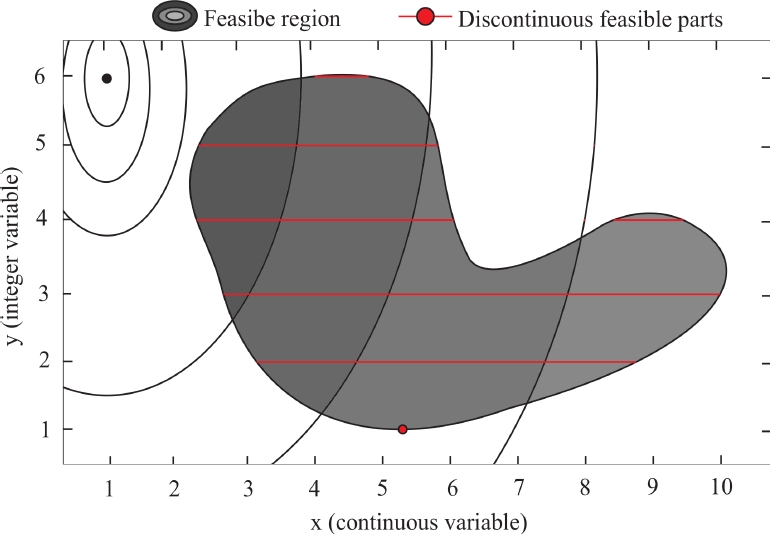
Fig. 1 MINLP problem example, where the shaded area represents the feasible region defined by the constraints, and the red lines are the discontinuous feasible parts that also satisfy the integer restrictions 

The shaded area is the feasible region defined by the constraints, and the red lines are the discontinuous feasible parts that also satisfy the integer restrictions.

In recent years, meta-heuristic optimization algorithm have gained popularity over classical MINLP techniques.

Different extensions of genetic algorithms [2], particle swarm optimization [4, 16], differential evolution [1, 5], ant colony optimization [13], harmony search [3], estimation of distribution algorithm [15], aimed at solving MINLP problems have been proposed.

The most significant advantage of these algorithms is their robustness regarding the function properties, such as non-convexity or discontinuities [12].

The classical MINLP techniques (like branch and bound, cutting planes, outer approximation) generally require prior convexification and relaxation operations, which are not always possible [11].

On the other side, when the population of meta-heuristic optimization algorithm converges to a discontinuous feasible part, it quickly loses diversity, and the exploration is reduced, with no possibility of jumping out to another discontinuous feasible part. Compared to larger discontinuous parts, it is difficult to find feasible solutions in the smaller parts. If the best solutions are located in small parts, then the population might converge to the wrong solutions.

Only a few recent works focused on MINLP problems consider the drawbacks described above. In [7], a multiobjective differential evolution is proposed.

This strategy gives equal priority to integer conditions and quality of the solution, and the population converges to good regions regarding both criteria.

In [6], the authors propose a cutting strategy that penalizes non-promising solutions, which means that non-promising parts are progressively discarded.

In addition, they propose a repulsion strategy that penalizes the discontinuous parts where the population is trapped, in order to search better solutions in other regions.

More recently, in [9] the Estimation of Distribution Algorithm for Mixed-Variable Newsvendor problem (EDAmvn) [15] is improved and proposed to MINLP problems.

The new proposal (EDAmv) uses the ε-constrained method to explore the smaller discontinuous feasible parts from infeasible contours. Also, the hybridization with a mutation operator is proposed.

In this work, we propose an algorithm, EDAIImv, with two modifications from the original EDAmv.

The first modification consists in establishing the exploration and exploitation components for the histogram of discrete variables, using the balance between both terms to improve the performance of the algorithm during the evolution.

The second modification is a repulsion operator to overcome the population stagnation in discontinuous parts, and continue the search for possible solutions in other regions.

Through a comparative analysis, the individual contribution of each modification to the algorithm performance was verified. The performance of EDAIImv is significantly higher than those of the compared algorithms.

2 Estimation of Distribution Algorithm

EDAmv is an improved version of EDAmvn, originally proposed in [15]. It uses an Adaptive-Width Histogram (AWH) model for handling continuous variables, and an ε-linked Learning-Based Histogram (LBHε) model for handling discrete variables.

New variable values are generated from statistical sampling. In the case of continuous variables, statistical sampling is hybridized with a mutation operator.

The replacement mechanism to get the next population is carried out through parent-offspring competition using the ε-constrained method.

2.1 Adaptive-width Histogram Model

The AWH model promotes promising regions by assigning them high probabilities, while in the other regions very low probabilities are assigned. One AWH is developed for each decision variable independently.

The search space [ai,bi] of the ith variable xi is divided into (W+2) bins (regions), to define the probabilities Pric for the AWH model.

Points [pi,0,pi,1,,pi,w+1,pi,w+2] define the width of the bins shown in Fig. 2, where pi,0=ai and pi,w+2=bi (ai and bi are the lower and upper bounds of xi, respectively).

Fig. 2 Search progress of the AWH model for W = 3. (a) first generations, (b) later generations 

The total number of bins is (W+2) although the input parameter for EDAmv is W , since the algorithm creates two more bins: one between the lower boundary ai and the point pi,1, and another one between the point pi,w+1 and the upper boundary bi (unpromising regions).

By assuming that xi,min1 and xi,min2 are the smallest and the second smallest existing values of variable xi, respectively, and xi,max1 and xi,max2 are the highest and the second highest existing values of variable xi, respectively, then points pi,1 and pi,w+1 are defined as in (7) and (8):

pi,1=max{xi,min10.5(xi,min2xi,min1),pi,0}, (7)

pi,w+1=min{xi,max1+0.5(xi,max1xi,max2),pi,w+2}, (8)

The W bins of the promising areas are located in the range [pi,1,pi,w+1], and have the same width a, given by (9):

a=(pi,w+1pi,1)W. (9)

Let Ai,j be the count of individuals for the ith variable located in the jth bin. As can be seen in Fig. 2, the end bins do not contain solutions (unpromising regions), then Ai,1=Ai,W+2=.

However, a small value will be assigned through the parameter eb, to avoid premature convergence. Ai,j is obtained by (10):

Ai,j{Ai,j,if2j(W+1,)eb,ifj=1,(W+2),andpi,j>pi,j1,0,ifj=1,(W+2),andpi,j=pi,j1. (10)

The first case in (10) is the count of bins of promising regions [pi,1,pi,w+1]. The second case corresponds to unpromising regions with ebvalue.

The third case assigns zero to the end bins with empty range. The probability of the ith variable in the jth bin is obtained by (11):

Pri,jc=Ai,jk=1W+2Ai,k. (11)

2.2 Learning-based Histogram Model Linked with ε-constrained

The LBHε model is used for handling integer variables. It is a link between the LBH model and the ε-constrained method.

The aim is to maintain an equal probability for all available integer values until ε reaches a predefined value εp, as is shown in Fig. 3 (a).

Fig. 3 LBHε model for v = 6. (a) ε>εp equal probability for all available integer values, (b) εεp considering population distribution 

When ε reaches εp, the LBH model begins the learning process, i.e., considering the information of the population distribution to update the probability, as shown in Fig. 3 (b).

If the ε-constrained method has been effective, for values of ε sufficiently small, the solutions must be close to those parts of the feasible region with promising objective function values.

Therefore, if the histogram begins the learning process at that point, it has a better chance of converging to good solutions.

Considering that the variable ym has v available integer values, with v{Lm,Lm+1,Lm+2,,Um}, the probability of the nth available value of v is defined by (12):

Prm,vd(t)={1(UmLm+1),ifε>εp,(1γ)Prm,vd(t1)+γCountvN,ifεεp. (12)

where N is the population size, t is the current generation, γ is the population learning rate, and Countv is the number of individuals with the nth available value of v.

Let lmax be the maximum number of generations, and γ a dynamic parameter defined by (13):

γ=ttmax. (13)

Therefore, as the number of generations advances, γ gradually increases as well, which implies an accelerated learning process, i.e., the model uses more information of the current population distribution.

2.3 Sampling

After the histograms have been developed, the offspring is obtained by sampling the models.

In case of a continuous variable xi, a bin j is firstly selected according to a randomly generated probability, then xi is uniformly sampled from the points that limit the bin selected [pi,j1,pi,j).

For a discrete variable ym, an available value of v{Lm,Um} is selected by a randomly generated probability.

2.4 Hybridization with a Mutation Operator

The mutation operation is added to generate the real variables. The vector of real variables x of each offspring is generated by mutation or by sampling taking into account the predefined mutation probability rM, i.e. if this probability is satisfied for a solution vector, its real variables are computed as shown in (14) and (15):

xk,ig+1=xbest,ig+β(xbest,igxk,ig), (14)

β=βmin+randk,i(βmaxβmin), (15)

where k,i are the index of the current solution vector and current variable, respectively, g is the current generation, xbest,ig is the ith variable of the best solution vector found so far, randk,i is a random number between 0 and 1, and βmin and βmax are the lower and upper bounds of β predefined by the user, with values between 0 and 1.

In the new proposal the values of βmin and βmax will always be set to 0 and 1, respectively.

2.5 Constraint Handling

The replacement mechanism to get the next population is carried out through parent-offspring competition using the ε-constrained method.

The ε-constrained method was proposed by Takahama and Sakai [14] as a constraint-handling technique.

Given two function values f(x1), f(x2), and two constraint violations ϕ(x1), ϕ(x2) for two points x1 and x2, the ε-constrained method uses the ε-level comparisons described in (16):

(f1,ϕ1)ε(f2,ϕ2)={f1f2,ifϕ1,ϕ2ε,f1f2,ifϕ1=ϕ2,ϕ1<ϕ2,otherwise, (16)

where ε-level comparisons are defined as an order relation on a pair of objective function and constraint violation values (f(x),ϕ(x)).

This means that the candidates with a violation sum lower than ε are considered as feasible solutions and are ordered according to their fitness values.

In the case of ε=0, ϕ(x) always precedes f(x). Therefore, this method favors the approach to the feasible region by keeping slightly infeasible solutions with promising fitness values.

The ε-level decreases at each iteration G until the predefined iteration number Tc is reached, after that ε=0, as indicated by (18):

ε(0)=ϕ(xθ), (17)

ε(G)={ε(0)(1GTc)cp,if0<G<Tc,0,otherwise, (18)

where cp is a parameter to control the speed of constraint relaxation, ε(0) is the initial value of ε, and xθ is the top θth in an array sorted by total constraint violation (θ=0.2N).

3 Proposed Method

Two modifications for EDAmv are proposed.

The first proposed modification focuses on establishing a new balance between exploration and exploitation of the LBHε model, in order to contribute to the algorithm performance during evolution.

The second modification is based on the repulsion of discontinuous parts that stagnate the population, with the aim of seeking better solutions in other discontinuous parts.

3.1 LBHε Improvement

As described in (12), γ is the learning rate of the population. A high value of γ increases the role of the population distribution Countv/N in obtaining the Prmd(t), whereas a low value mainly considers the histogram of the previous generation, Prmd(t1).

However, when certain admissible values begin to prevail statistically over others, the histograms and the populations begin to be similar, so the terms of the equation (12), instead of combining different information, emphasize the same search direction and cause accelerated (and often premature) convergence.

In this work, the following LBHε model is proposed:

Prm,vd(t)={Pem,vd,ifε>εp,(1γ)Pem,vd+γCountvN,ifεεp, (19)

where Pemd are equal probabilities for all v values of the mth variable, and are given by (20):

Pem,vd=1(UmLm)+1. (20)

In this model, Pemd contributes to the exploration of the algorithm, while Countv/N contributes to the exploitation on the most populated regions (promising regions).

As can be seen in Fig. 4, now for very low values of γ, the histogram will be flatter (low selection pressure).

Fig. 4 LBHε model, γ=0 random exploration, γ=0.5 middle consideration of population distribution, γ=1 total consideration of population distribution 

As the value of γ increases, the histogram and selection pressure will be more consistent with the population distribution. As in the previous case, γ is a dynamic parameter defined by (13).

3.2 Repulsion

The repulsion strategy proposed in [6] consists of two steps: (i) judge whether the population is trapped into a solution, and (ii) apply a repulsion operator to the discontinuous feasible part containing the solution, and restart the population. Eq. (21) is the fail consideration to find a better solution:

(fbestfbest)0&amp;(gbestgbest)0, (21)

where fbest and gbest are the objective function value and the degree of constraint violation of the best solution found so far, respectively, fbest and gbest are the objective function value and the degree of constraint violation of the best solution in the current generation, respectively.

If (21) is satisfied, it means that the algorithm fails to find a better solution, then the counter is incremented (ctr=ctr+1). If (21) is not satisfied in any generation, the counter is reset (ctr=0).

If ctr is greater than a predefined failure threshold T, the population is considered to be trapped in a solution, and the discontinuous feasible part (y) containing that solution has been explored. Then the population is regenerated, and the solution is recorded in the store archive. Any population member that has a vector y contained in store will be penalized with an arbitrarily large degree of constraint violation.

ε-constrained method is also restarted but with a new Tc value with fewer generations, called fast generation control (Tc). At the end of the execution, the recorded solutions should be considered to return the best solution.

4 Experimentation and Results

4.1 Benchmark Problems

Sixteen MINLP problems (F1-F16) were used to evaluate the performance of EDAIImv. Because of the space limitation, a detailed description of the problems is not included, but it can be found in [6].

The maximum number of objective function evaluations was set at 200,000, and 25 independent runs were executed for each problem. The tolerance value for the equality constraints was set at 1.0E-04.

A run was considered as successful if: |f(xbest)f(x*)| 1.0E-4, where x* is the best known solution and xbest is the best solution provided by the algorithm.

4.2 Algorithms and Parameter Settings

PSOmv [16], EDAmv [9], and EDAIImv were the competing algorithms in the experiment. PSOmv also uses the LBH model for handling discrete variables. However, the γ is an adaptive parameter, and the LBH probability is updated using only the best half of the swarm.

To prove the individual contribution of each modification proposed, the instance with only LBHε improvement (EDAmv(I)) was also included. The algorithms were tuned using the iRace parameter tuning tool [8]. The parameter values were as follows:

PSOmv: swarm size N=300, acceleration coefficient c=1.5299, learning rate γ=0.0125.

EDAmv: N=50, numbers of bins W=4, end bins parameter eb=2.3959, control generation Tc=3,000, control speed parameter cp=8, link parameter εp=0.2399, and mutation parameters: rM=0.6, βmin=0.3, βmax=0.9.

EDAmv(I): N=50, W=3, eb=2, Tc=2000, cp=7, εp=5, and rM=0.3.

EDAIImv: N=50, W=3, eb=2, Tc=2000, cp=7, εp=5, rM=0.3, failure threshold T=400, and fast control generation Tc=200.

4.3 Analysis of Results

Table 1 summarizes the results of PSOmv, EDAmv, EDAmv(I), and EDAIImv.

Table 1 PSOmv, EDAmv, EDAmv (I), and EDAIImv results 

Problem Status PSOmv EDAmv EDAmv(I) EDAIImv
F1 FR 100 100 100 100
SR 0 100 0 100
Ave ± Std Desv 17.000±0.000 + 13.000±0.000 17.000±0.000 + 13.000±0.000
F2 FR 100 100 100 100
SR 100 100 100 100
Ave ± Std Desv 1.000±0.000 1.000±0.000 1.000±0.000 1.000±0.000
F3 FR 100 100 100 100
SR 24 100 76 100
Ave ± Std Desv -3.879±0.217 + -4.000±0.000 -3.880±0.218 + -4.000±0.000
F4 FR 100 100 100 100
SR 100 100 100 100
Ave ± Std Desv -6.000±0.000 -6.000±0.000 -6.000±0.000 -6.000±0.000
F5 FR 100 100 100 100
SR 0 100 76 100
Ave ± Std Desv 1.240±0.000 + 0.250±0.000 0.488±0.432 + 0.250±0.000
F6 FR 100 100 100 100
SR 100 100 100 100
Ave ± Std Desv -6,783.582±0.000 -6,783.582±0.000 -6,783.582±0.000 -6,783.582±0.000
F7 FR 96 100 100 100
SR 0 24 28 36
Ave ± Std Desv NA + 0.895±0.235 + 0.725±0.361 + 0.642±0.359
F8 FR 100 92 100 100
SR 0 0 0 0
Ave ± Std Desv 7,222.847±94.800 -NA + 7,971.856±518.086 7,986.723±906.139
F9 FR 100 88 100 100
SR 16 0 0 0
Ave ± Std Desv 7,284.444±283.224 -NA + 8,305.496±742.746 8,391.061±854.267
F10 FR 100 64 96 100
SR 64 0 0 0
Ave ± Std Desv 7,337.332±277.610 -NA + NA + 8,086.671±641.101
F11 FR 100 100 100 100
SR 0 0 0 0
Ave ± Std Desv 46.280±6.601 + 40.785±5.484 + 38.119±5.378 37.822±5.334
F12 FR 100 100 100 100
SR 0 0 0 4
Ave ± Std Desv 90.048±17.975 + 74.500±30.941 + 51.976±20.146 56.201±23.594
F13 FR 100 100 100 100
SR 0 0 0 4
Ave ± Std Desv 8,956.649±7.448 8,943.236±29.864 8,955.137±31.467 8,949.792±35.701
F14 FR 100 100 100 100
SR 0 48 60 76
Ave ± Std Desv 8,977.707±66.813 + 8,963.673±41.007 8,954.966±10.181 8,958.233±41.392
F15 FR 100 100 100 100
SR 0 0 0 0
Ave ± Std Desv 30.899±1.203- 34.997±3.938 + 30.580±1.827 31.639±2.105
F16 FR 100 100 100 100
SR 0 0 0 0
Ave ± Std Desv 31.086±0.001 -51.652±23.202 + 31.598±1.353 ≈ 31.636±1.365
[+/=/] [7/4/5] [8/8/0] [5/11/0] —–

These results are assessed considering the terms Feasible Rate (FR), Successful Rate (SR), Average (Ave), and Standard Deviation (Std Dev), over 25 independent runs. “NA” means that an algorithm cannot achieve 100% FR.

EDAmv(I) beats EDAmv in nine problems (F7:F12, F14:F16) in at least one of the term concerned, proving that LBHε has a positive influence on the algorithm performance.

As mentioned above, the LBH model (used in EDAmv) has two terms that could contain redundant information, producing an accelerated convergence.

However, for problems F1, F3, and F5, where the solutions are in small feasible parts, a slower convergence of LBHε (used in EDAmv(I)) causes that the ε-level reaches zero value when the histogram has not yet converged to the small promising part.

The repulsion strategy is very useful for this situation, since restarts the exploration in the remaining unexplored parts.

As can be seen, the implementation of repulsion strategy in EDAIImv improves the performance for problems F1, F3, and F5 without compromising the rest of the problems.

A Wilcoxon’s rank-sum test at a 0.05 significance level was carried out between EDAIImv and each competitor, in order to evaluate the significant differences in the results.

In Table 1, [+], [] and [] denote that EDAIImv is better than, worse than, and similar to its current competitor, respectively.

As shown in the final part of Table 1, the results of EDAIImv are significantly better than EDAmv in eight problems (F7:F12, F15,F16), similar in another eight problems (F1:F6, F13, F14), and in no case EDAmv surpasses the result of the new proposal.

EDAmv(I) results are outperformed on five problems (F1, F3, F5, F7, F10), matched on eleven problems (F2, F4, F6, F8, F9, F11:F16), and in no case is EDAIImv outperformed by EDAmv(I).

It is clear that EDAIImv has significantly better results than previous variants. Analyzing the results of this sequenced implementation, it can be concluded that each proposed modification contributes to a better performance.

Regarding PSOmv, the new proposal is significantly better in seven test problems (F1, F3, F5, F7, F11, F12, F14) and no difference in four problems (F2, F4, F6, F13), while PSOmv outperformed EDAIImv in five problems (F8, F9, F10, F15, F16).

Although in general EDAIImv has a better performance than PSOmv, the advantage of PSOmv in the last mentioned problems is due to a superior diversity in the exploration.

Therefore, it is recommended in future works to focus on promoting greater diversity in EDAIImv.

5 Conclusion and Future Work

EDAIImv was proposed with two modifications regarding its previous version EDAmv.

The first modification establishes a better balance between the exploration and exploitation terms in LBHε, aimed at improving the performance of the algorithm during the evolution.

The second modification is a repulsion operator to overcome the population stagnation in discontinuous parts, and continue the search for good solutions in other regions.

Through a comparative analysis on sixteen test problems, the individual contribution of each modification to the algorithm performance was verified.

According to the Wilcoxon’s rank-sum, EDAIImv showed significantly better performance than its previous version.

The benchmark was also used to compare the performance of the improved proposal against PSOmv. Overall, EDAIImv has a better performance than PSOmv.

However, PSOmv presents an advantage in some problems due to a superior diversity in the exploration. Therefore, it is recommended in future works to focus on promoting higher diversity in the EDAIImv.

First and third authors acknowledge support from SIP-IPN through project No. 20221928.

Fourth author acknowledges support from SIP-IPN through project No. 20221960.

Acknowledgments

The first author acknowledges support from the Mexican National Council of Science and Technology (CONACyT) through a scholarship to pursue graduate studies at the CIDETEC-IPN.

References

1. Datta, D., Figueira, J. R. (2013). A real–integer– discrete-coded differential evolution. Applied Soft Computing, Vol. 13, No. 9, pp. 3884–3893. DOI: 10.1016/j.asoc.2013.05.001. [ Links ]

2. Deep, K., Singh, K. P., Kansal, M. L., Mohan, C. (2009). A real coded genetic algorithm for solving integer and mixed integer optimization problems. Applied Mathematics and Computation, Vol. 212, No. 2, pp. 505–518. DOI: 10.1016/j.amc.2009.02.044. [ Links ]

3. Lee, K. S., Geem, Z. W., Lee, S.-h., Bae, K.-w. (2005). The harmony search heuristic algorithm for discrete structural optimization. Engineering Optimization, Vol. 37, No. 7, pp. 663–684. DOI: 10.1080/03052150500211895. [ Links ]

4. Li, L., Huang, Z., Liu, F. (2009). A heuristic particle swarm optimization method for truss structures with discrete variables. Computers & structures, Vol. 87, No. 7-8, pp. 435–443. DOI: 10.1016/j.compstruc.2009.01.004. [ Links ]

5. Lin, Y., Liu, Y., Chen, W. N., Zhang, J. (2018). A hybrid differential evolution algorithm for mixed-variable optimization problems. Information Sciences, Vol. 466, pp. 170–188. DOI: 10.1016/j.ins.2018.07.035. [ Links ]

6. Liu, J., Wang, Y., Huang, P. Q., Jiang, S. (2021). Car: A cutting and repulsion-based evolutionary framework for mixed-integer programming problems. IEEE Transactions on Cybernetics. DOI: 10.1109/TCYB.2021.3103778. [ Links ]

7. Liu, J., Wang, Y., Xin, B., Wang, L. (2021). A biobjective perspective for mixed-integer programming. IEEE Transactions on Systems, Man, and Cybernetics: Systems, Vol. 52, No. 4, pp. 2374–2385. DOI: 10.1109/TSMC.2020.3043642. [ Links ]

8. López-Ibáñez, M., Cáceres, L. P., Dubois-Lacoste, J., Stutzle, T. G., Birattari, M. (2016). The irace package: User guide. IRIDIA, Institut de Recherches Interdisciplinaires et de Developpements en Intelligence Artificielle, Universite Libre de Bruxelles. [ Links ]

9. Molina-Pérez, D., Portilla-Flores, E. A., Mezura-Montes, E., Vega-Alvarado, E. (2022). An improved estimation of distribution algorithm for solving constrained mixed-integer nonlinear programming problems. IEEE World Congress on Computational Intelligence, IEEE, pp. 1–8. DOI: 10.1109/CEC55065.2022.9870338. [ Links ]

10. Ponsich, A., Azzaro-Pantel, C., Domenech, S., Pibouleau, L. (2007). Mixed-integer nonlinear programming optimization strategies for batch plant design problems. Industrial & engineering chemistry research, Vol. 46, No. 3, pp. 854–863. DOI: 10.1021/ie060733d. [ Links ]

11. Sahinidis, N. V. (2019). Mixed-integer nonlinear programming 2018. Optimization and Engineering, Vol. 20, No. 2, pp. 301–306. DOI: 10.1007/s11081-019-09438-1. [ Links ]

12. Schlueter, M. (2012). Nonlinear mixed integer based optimization technique for space applications. Ph.D. thesis, University of Birmingham. [ Links ]

13. Schluter, M., Egea, J. A., Banga, J. R. (2009). Extended ant colony optimization for non-convex mixed integer nonlinear programming. Computers & Operations Research, Vol. 36, No. 7, pp. 2217–2229. DOI: 10.1016/j.cor.2008.08.015. [ Links ]

14. Takahama, T., Sakai, S. (2006). Constrained optimization by the ε constrained differential evolution with gradient-based mutation and feasible elites. IEEE international conference on evolutionary computation, IEEE, pp. 1–8. DOI: 10.1109/CEC.2006.1688283. [ Links ]

15. Wang, F., Li, Y., Zhou, A., Tang, K. (2019). An estimation of distribution algorithm for mixed-variable newsvendor problems. IEEE Transactions on Evolutionary Computation, Vol. 24, No. 3, pp. 479–493. DOI: 10.1109/TEVC.2019.2932624. [ Links ]

16. Wang, F., Zhang, H., Zhou, A. (2021). A particle swarm optimization algorithm for mixed-variable optimization problems. Swarm and Evolutionary Computation, Vol. 60, pp. 100808. DOI: 10.1016/j.swevo.2020.100808. [ Links ]

Received: July 06, 2022; Accepted: September 19, 2022

* Corresponding author: Efrén Mezura-Montes, e-mail: emezura@uv.mx

Creative Commons License This is an open-access article distributed under the terms of the Creative Commons Attribution License