


 text new page (beta)
 English (pdf)
 Article in xml format
 Article references
 Send this article by e-mail
 Cited by SciELO
  Similars in
SciELO
Similars in
SciELO 
 Permalink
1 Introduction
Detecting Cardiovascular Diseases (CVDs) prematurely is of great interest for the Healthcare Industry. According to the World Health Organization (WHO), almost 18M deaths, representing 32% of global deaths in 2019 were caused by heart diseases, as part of CVDs [6]. Furthermore, 75% of these cases took place in low or middle income countries, not to mention that 38% of premature deaths (under the age of 70) were caused by CVDs [6].
On top of that, Centers for Disease Control and Prevention (CDC) claim that about half of USA’s population has at least one of three risk factors for CVD [9]: high blood pressure, high cholesterol and smoking. With that in mind, CDC [3] surveyed American citizens all over the country which led to a data set containing almost 400k observations, whether the person in question has ever been diagnosed either with Coronary Heard Disease or Myocardial Infarction.
Even though several approaches on how to detect these kind of disease using Machine Learning (ML) have been developed through out recent times, in this work we aim to find a robust yet interpretable way of finding out which risk factors are more strongly correlated with CVDs, particularly Coronary Heart Disease and Myocardial Infarction.
To pursue our goal, we use a public dataset from the CDC to test three different ML models. We defined the importance of features in order to select the most relevant ones. Through a benchmark among these models, we determined the best model. Lastly, we implemented the best model in an easy application that can be used in preventing the detection of CVDs.
Here we aim not only to find an accurate predictor but to examine which risk factors are more closely related to CVD detection, leading to prevention or better and early management.
The rest of the paper is organized as follows. Section 2 summarizes the related work. Section 3 presents the methodology implemented in this work, from the data collection, data preparation, training models, and evaluation of models.
Section 4 shows the experimental results and the implementation in an application. Lastly, Section 5 concludes the paper.
2 Related Work
Various efforts have been made towards finding out which is the best, most accurate model for CVD detection. In 2018, the work in [8] showed how Decision Trees might not be a great candidate by themselves as it’s quite hard not to over-fit, while Support Vector Machines (SVM) can easily outperform Decision Trees and Random Forest or Ensemble Methods can perform well too.
Complementing these results, the authors in [5] have shown how different models performed better while coupled with different over sampling techniques. Particularly, it was found that Synthetic Minority Oversampling was the best match for Random Forest, SVM and Random Over Sampling work great together, too. Also, Adaptive Synthetic Sampling helped, once again, Random Forest gets the best results.
The latter is very relevant as it turns out some other works have been done around finding out which tree-based models work better on CVD detection. Using a data set from UCI Machine learning repository, the authors in [7] found that J48 is the best technique for CVD detection amongst some other well-known tree-based methods.
3 Methodology
In this work, we implement the overall workflow for achieving the CVD estimation using ML models, depicted in Fig. 1. This workflow consists of four main steps: data collection, data preparation, training models, and evaluation of models.

3.1 Dataset Description
The dataset used for this study, was downloaded from Kaggle repository. Originally, it comes from the CDC’s (Centers for Disease Control and Prevention) Behavioral Risk Factor Surveillance System [2] which conducts telephone surveys about the health status of USA’s citizens and contained around 300 features. It has been pre-processed and cleaned. So that in this work, we use the smaller data set with 18 features.
The dataset is divided into 13 categorical variables, 4 numerical variables and one categorical target (‘HeartDisease’), consisting of 319,795 records without null values; but it is heavily unbalanced. Table 1 represents the frequency of the most common category on each categorical feature, while Fig. 2 represents the distribution of the four numerical variables.
Table 1 Categorical variables in the dataset
| Feature | Categories | Top Category | Frequency |
| HeartDisease | 2 | No | 292422 |
| Smoking | 2 | No | 187887 |
| AlcoholDrinking | 2 | No | 298018 |
| Stroke | 2 | No | 307726 |
| DiffWalking | 2 | No | 275385 |
| Sex | 2 | Female | 167805 |
| AgeCategory | 13 | 65-69 | 34151 |
| Race | 6 | White | 245212 |
| Diabetic | 2 | No | 269653 |
| PhysicalActivity | 2 | Yes | 247957 |
| GenHealth | 5 | Very Good | 113858 |
| Asthma | 2 | No | 276923 |
| KidneyDisease | 2 | No | 308016 |
| SkinCancer | 88 | 788 | 289976 |
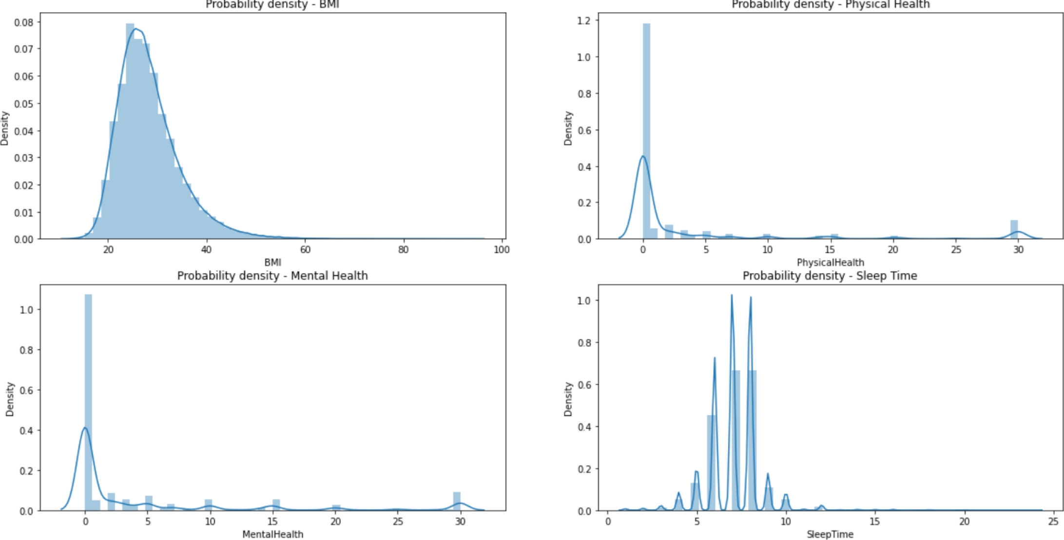
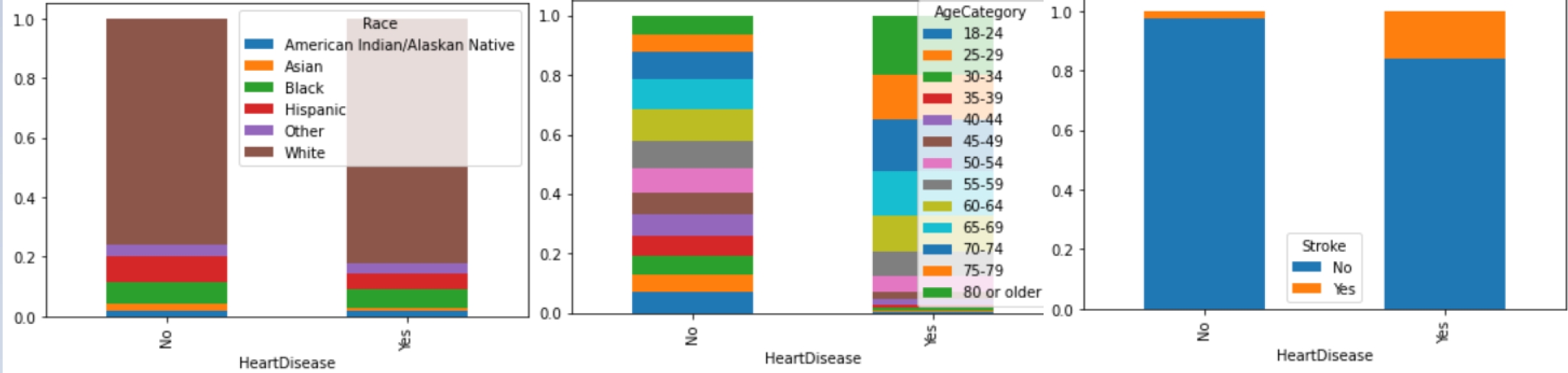
Figure 3 shows an example of the relationship between the variables and the target. We know that the number of observations are 319,795, of those 292,422 belong to the negative class. Thus, it is important to balance the data.
3.2 Data Pre-Processing
As we are dealing with both categorical and numerical variables on top of an imbalanced dataset, we must have at least three pre-processing tasks to do:
— Perform One-Hot encoding on categorical variables.
— Perform standard scaling to numerical variables.
— We use over sampling and under sampling to balance classes.
For feature preparation, we decided to use the sklearn pre-processing module on Python, OneHotEncoder and StandardScaler, to perform the first part of the process. Then, for re-sampling, we have used RandomOverSampler and RandomUnderSampler for balancing the classes. And, finally, we split the data in training and holdout sets.
After the EDA we know the data types of the variables, we created a pipeline. The first step was to normalize all numeric features using an standard scaler, for categorical values we used One-Hot encoding, and last we used a label encoder for the target feature. Imputing of null values was not necessary because we did not have any empty values.
Next, we separated the dataset in 80% of training data and 20% of testing data. It is remarkable to say that we stratified the data to assure all the target values were distributed in both train/test sets.
The third step consisted on balancing the target feature because originally we had a ratio of 91 vs 9 of the negative and positive classes respectively. We did a random over-sampling to get a relationship of
3.3 Building Models
We decided to test three different model classifiers: Stochastic Gradient Descent Based (SGD) Classifier, Logistic Regression, and Random Forest.
We decided to use Optuna [1] for hyper-parameter tuning, which is an open source hyper-parameter optimization framework to automate hyper-parameter search more efficiently. One of the key reasons we decided to use this library is because it is able to do automated search for optimal hyper-parameters using Python conditionals, loops, and syntax. It also uses state-of-the-art algorithms which help to efficiently search large spaces and prune unpromising trials for faster results. In the basis, it uses Bayesian optimization that builds a probability model of the wrapped objective function and uses it to select hyper-parameters to evaluate in the true objective function.
For the SGD Classifier, we use four different hyper-parameters such as alpha, penalty, loss, and max_iter. For the Logistic Regression model the hyperparameters used were: penalty, c value, solver, and fit_intercept. Lastly for the Random Forest Classifier, it used four different hyper-parameters such as max_depth, n_estimators, criterion, and max_features.
For hyper-parameter tuning, we implement a 3-fold 20-repetition cross validation technique. Table 2 summarizes the best hyper-parameters per model.
Table 2 Optimized hyper-parameters for the models
| Model | Hyperparameters |
| SGD Classifier | alpha=3.81E-5, penalty=‘elasticnet’, max_iter=60 |
| Logistic Regression | regularization=L2, reg_coefficient=45.52 |
| Random Forest | max_depth=38, n_estimators=299, criterion=gini, max_features=‘auto’ |
The following graphs shows the objective value for each trial ran by the optuna objective function, in this case, it only shows the top 10 trials. We can see that it starts with an objective value around 0.76 and after the fourth trial, it shows the best objective value with a value around 0.915.
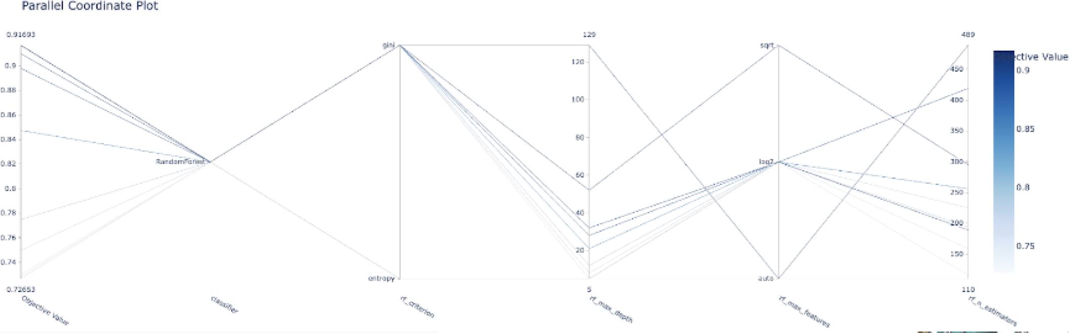
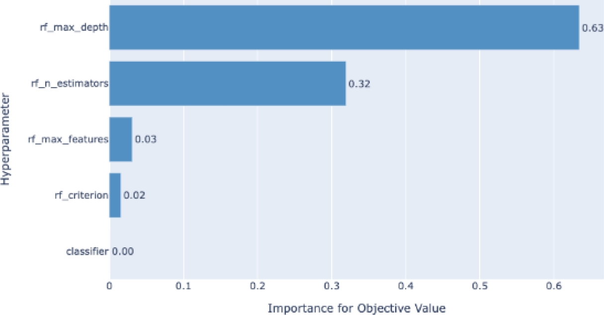
Figure 4 shows an example of the evolution of the model accuracy (objective function) based on the trials of the different combinations of the hyper-parameters. Another representation of the hyper-parameter evolution under the optimization process can be seen in Fig. 5. In addition, Fig. 6 shows an example of the influence of the hyper-parameters in the model accuracy (objective function). The latter would be interesting for better understanding on the role of the hyper-parameters in the building of the models.

3.4 Experimentation
In order to find the best algorithm, we first ran the hyper-parameter optimization process with Optuna. Then, the best classifier is selected in terms of the accuracy metric (1), where, TP, TN, FP, and FN represent true positive, true negative, false positive, and false negative, respectively:
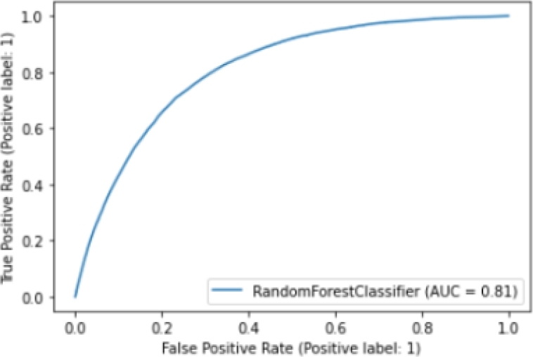
In addition, we plot the ROC (Receiver Operator Characteristic) curve [10], which helps us understand the trade-off between sensitivity and specificity. Classifiers that give curves closer to the top-left corner indicate a better performance.
4 Experimental Results
We conducted the training of the three model classifiers, and results are summarized in Table 3. It can be observed that the Random Forest model gets the best accuracy metric (94%).
Table 3 Results of the training models
| Model | Accuracy (%) |
| SGD Classifier | 76 |
| Logistic Regression | 80 |
| Random Forest | 94 |
Figure 7 shows the ROC curve of the Random Forest model. We find that our model has an AUC (Area Unders Curve) of 0.81, which is equivalent to the probability that a randomly chosen positive instance is ranked higher than a randomly chosen negative instance. Note that the ROC does not depend on the class distribution. This makes it useful for evaluating classifiers predicting rare events such as ours.
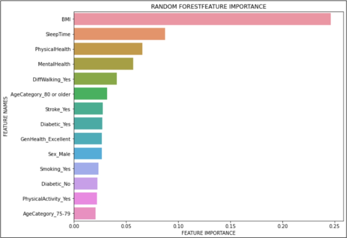
We also did a feature importance graph to find which variables are the most important ones for the model. Out of 41 different features, Fig. 8 only shows the fourteen most important features, such as body mass index (BMI), sleep time, physical health, mental health, among others.
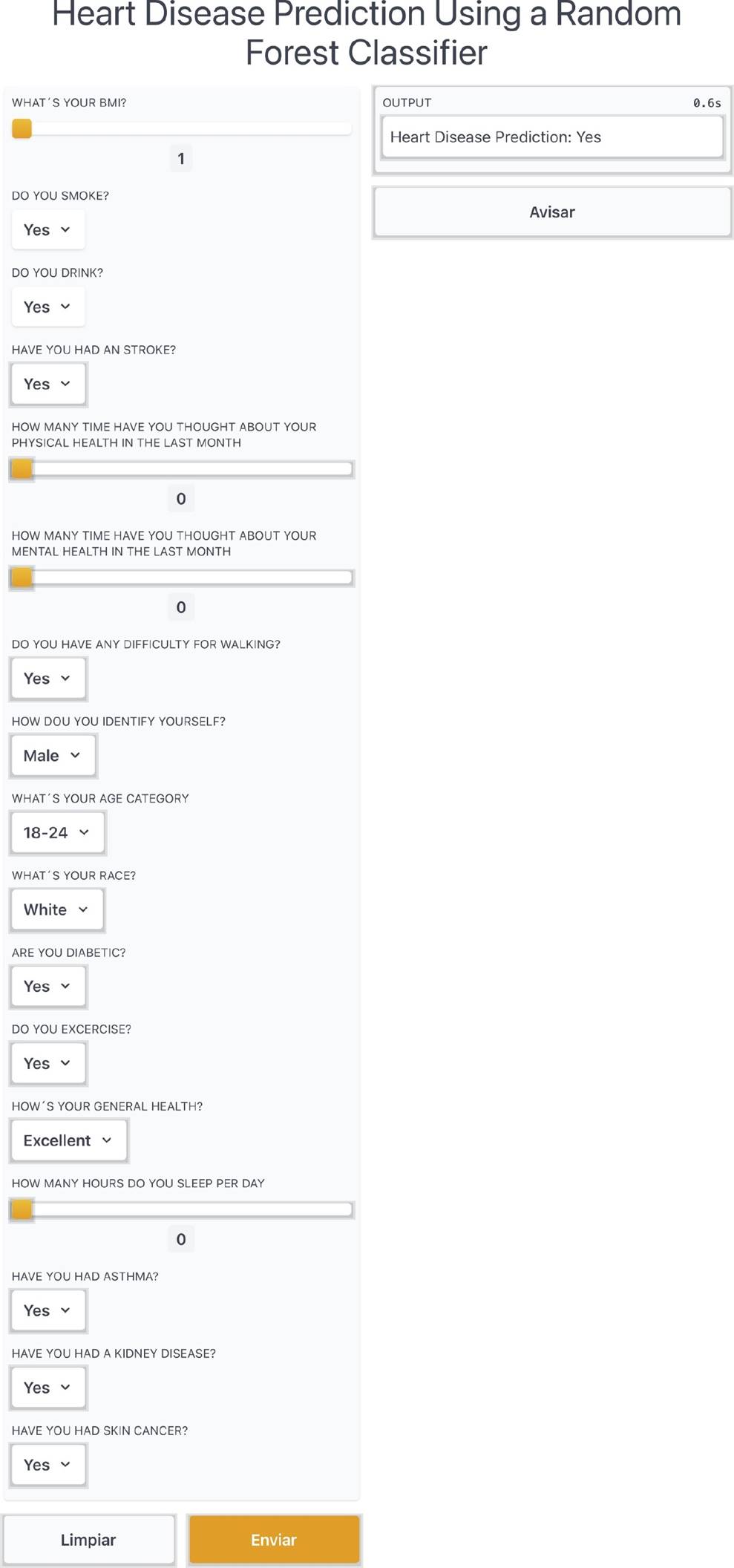
Furthermore, we created an application on Gradio library of Python in order to create a functional application to show our model. In the application, the user inputs the required parameters using a friendly interface, and those inputs are processed in order to obtain a quick result of the heart disease prediction of the person. Figure 9 shows an excerpt of the web application running the Random Forest classifier.
The results validate that our proposal consists of an ML model, to say Random Forest classifier, that is highly accurate (94% of accuracy) and robust enough for a medical application (81% of AUC). Furthermore, we find that the automatic detection of feature relevance (see Fig. 8) is consistent with the literature, in which BMI, sleep time, and physical health are the most common risk factors in CVDs [4].
In addition, we developed a web application tool based on the Random Forest classifier for heart disease estimation, leading to prevention or better and early management of the disease. This work is limited on the data used, since it looks biased in terms of gender and ethnicity, and the dataset is unbalanced too. So, it would be better to expand the investigation with more detailed and unbiased data. However, this work can confirm that this preliminary work might help facing CVD in patients.
5 Conclusions
This work proposed to build a robust yet interpretable way of finding out which factors are more strongly correlated with CVDs using machine learning models. To do so, we explored three ML classifiers, and we found that Random Forest model is the best for the dataset used.
It is evident that imbalance is a big problem for this data set on top on non-separability. Other techniques for imbalanced learning can be applied to this problem like class weights, using gradient boosting for a more robust sequential tree ensemble that would help better differentiate the binary classes. Using these techniques should result in better classification performance that could help in many cases. For instance, a Hospital could survey patients and find out whether they are candidates for CVD prevention treatment or feature importance could help pharmaceutical companies target specific drugs on their campaigns or simply.
Even though our model has a good performance, the model needs improvement. For future work, we can use other ML techniques and adding more features to our model for better complexity and understanding of the patient’s information. Other data sets can also be explored.

