


 text new page (beta)
 English (pdf)
 Article in xml format
 Article references
 Send this article by e-mail
 Cited by SciELO
  Similars in
SciELO
Similars in
SciELO 
 Permalink
Introduction
The vast amount of data (big data) produced within the healthcare industry is analyzed to provide better healthcare services to patients. The analytical system of big data is designed with very efficient integrated technology. Healthcare is one of the many big data applications that use both big data analytics and a relatively new well-known technology called deep learning to provide high-quality treatment to patients. Data gathered for healthcare informatics comes from different modalities MRI, fMRI, SPECT, PET, CT, and DTI. Using various deep learning algorithms with large amounts of healthcare data allows the healthcare industry to make more informed and faster decisions.
Recently MRI has been extensively utilized for the diagnosis of different diseases. This study aims to find the link between deep learning and the diagnosis of Alzheimer's patients.
Alzheimer's disease (AD) is the most common cause of dementia, and it is one of the currently leading diseases in most countries.
According to NIA, it will exceed the rate by 16 million in 2050 [1]. The unexpected growth of AD creates a huge economic breakdown for countries like USA and UK. According to the Alzheimer Association, 5.5 million Americans suffered from AD at the age of 65 or above.
Alzheimer's disease is named after Dr.Alois Alzheimer in1906 [2]. It is not a genetic disease but it happens due to two abnormal clumps called Amyloid plaques and tangles called tau protein. In the mid-60s, doctors found certain aspects of cognition, such as weak thinking power, behavioral changes, poor visuospatial ability, etc in an AD patient. By performing brain scans, such as MRI through effective radioglaciology approaches, a huge amount of imaging data is generated because each patient has thousands of medical images.
Due to this Big Data analytics was introduced with different characteristics. Here volume is one of the characteristics of big data managed and analyzed by different tools of both big data analytics and deep learning with its great advantages.
Here Fig. 1 shows a sagittal view of Alzheimer's pre-processed scan by Keras. In this paper, we proposed a novel method for the classification of Alzheimer's (AD) vs mild cognitive impairment in a prodromal stage of AD vs (MCI) vs healthy control (HC) by deep learning architecture. Deep learning tools have been applied to medical images for computer-aided pathology detection, classification, and prediction.

In recent, deep learning tools have been shown highly effective for a broad range of big healthcare analytics, multiple hidden layers are placed in between input and output layers for better analysis in diagnosing AD patients. For feature extraction, several hidden layers are placed, and each next layer contains the feature of the previous layer.
This paper pays close attention to the convolutional autoencoder for the diagnosis of AD. Combining both the approaches of CNN and Autoencoder for feature extraction of AD is our main motive behind this research. In this paper, we proposed a convolutional autoencoder deep learning for unsupervised feature learning to improve accuracy.
The remaining section is organized as follows. Section 2 contains an elaborative description of related works. Section 3 describes the convolutional neural network. Section 4 describes the proposed convolutional autoencoder (CANN) model. Section 5 elaborates on the comparisons between the two techniques of convolutional autoencoder (CANN) and Independent component analysis (ICA). Section 6 presents the experiment and result in part. Section 7 elaborates the classification part. Section 8 gives the discussion part and the last section contributes the conclusion part.
2 Related Work
To classify patterns, selecting a subset of an input variable from a whole set of the learning algorithm is the motivation for feature extraction:
{f1,f2,f3,fu……fm}→{fij…fuv,…,fun},uv∈{1,…,m},v=1,…,n.
Feature selection makes more accuracy a model if the feature is very large. By overcoming traditional methods of feature selection algorithms like filter method, wrapper method, and embedded methods, deep learning approaches were introduced to get a higher accuracy through big healthcare data.
The manual approaches of radiologists are more complex to degenerate features for better detection. A large amount of unlabeled data is used to learn the features in unsupervised learning approaches.
Convolutional neural network (CNN) has been creating good research on text analysis, image detection, speech recognition, etc. in the field of deep learning. Many researchers have shown that CNN is better to extract features as compared to the traditional method like SVM [3] finding the classification of skin concern with the deep neural network.
Unsupervised methods are an effective research area for using SAEs to classify AD & MCI [4]. For classification of AD using a whole-brain hierarchical network [5] was very well defined in their research, paper.AD classified the AD via a deep convolutional neural network using MRI & fMRI data [6] is also a landmark for feature study.
3 Convolutional Neural Network (CNN)
Image segmentation is becoming a critical/different challenge for clinical researchers using machine-learning technologies. As a result, various distinct works in the medical area are currently giving a location for research to overcome the difficulty of high dimensionality data through segmentation.
Despotovic et al. [7] provided a substantial review of the different segmentation techniques. All proposed segmentation technique deploys on evolutionary algorithms. Diverse strategies are presented to briefly define the task to increase performance based on the different anatomy and functions of medical images.
In addition, using deep learning to combine high-dimensional data, such as massive medical data, different feature selection/extraction or to generate disease characteristics for a better diagnosis is possible.
The training model for medical imaging classification typically takes one or more images as inputs and outputs yes or no.
CNN was first used in image analysis in 2012 as a faster and more accurate model. The real definition of convolution, in general, is the integral of the product of two signals:
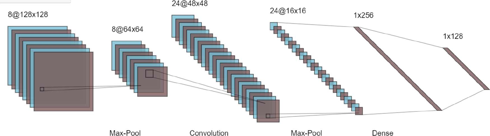
The different layer of CNN is the convolutional layer, rectified linear unit (RELU) layer, and pooling layer are described in Fig. 1.
To extract text characteristics or procure the features of any disease is simpler for researchers by using CNN techniques.
Here Fig. 2 briefly describe the different layer with the proper equation.
3.1 Convolutional Layer
The VGG (visual geometry Group) has established a track for classification. The whole-brain image is fed into CNN, which uses hidden layers to extract useful characteristics. The first function contains input values as pixel values, whereas the second function contains the kernel as a filter.
The dot product among two functions gives output as another function, and the filter is shifted over the image from one position to another is called stride length for detecting real features.
The feature map (activation) is captured by shifting the operation by covering the entire image. The CNN has a limited connection to the next layer for meaningful feature detection. The ‘*’ is denoting the convolutional operation. Other notation is as following.
Output feature map=l(t).
l(t)=h(t)*k(t)=(h*k) (t):
l: denoted as output or feature map.
t: denoted as integer.
h: denoted as input.
k: denoted filter or kernel.
*: convolutional operation.
Discretized convolutional formula:
l(t)=∑bi(b)∗k(t−b).
For two dimensions:
l(t)=∑a∑bi(a,b)∗k(u−a,v−b).
3.2 RELU Layer
In the Relu layer, replace the - ve values with 0 for avoiding the vanishing gradient problem.
P(x)=max (0, x).
x→input to the neuron.
Among all the activation functions, Relu is one of them to maintain the CNN operation.
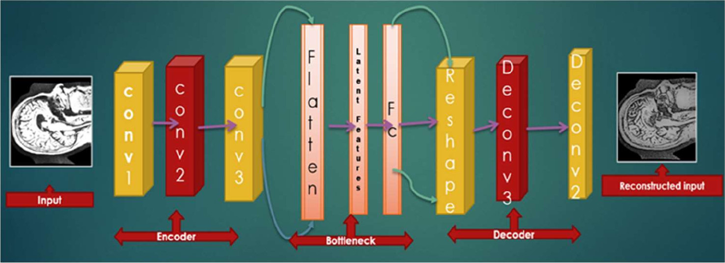
4 Proposed Convolutional Autoencoder Model
To build a better model, MRI images are very useful for the classification of medical data. From a supervised point of view, weights are updated through forwarding and backward propagation. Standard autoencoder is the artificial neural network and for the unsupervised convolutional filter, convolutional autoencoder (CAE)is a tool that learns to encode input and tries to reconstruct the input by decoding layer.
The raw AD MRI patches are input to the convolutional autoencoder CANN for feature learning and the explicit parameters are determined by autoencoder’s unsupervised learning. CNN is then classified by classification technique.
CAE is the type of CNN, where filters are learning and aim to classify the inputs. At first, it is the autoencoder (AE) that uses both the convolutional and pooling layer to extract the hidden pattern of input features. In the decoding phase, deconvolutional and unpooling for reconstructing the features from the hidden pattern. Specifically, the different patches of AD MRI images can be denoted as:
U∈U.
U⊂Rn∗l∗l.
n→no. of input channels.
l∗l→size of input images.
unlabeled dataset=UD--={u|u∈U}.
4.1 Autoencoder
Specifically, the standard autoencoder is based on a supervised learning approach. If we explained the autoencoder technique, our aim of this paper is fully solved.
The Autoencoder technique is a type of artificial neural network (ANN), which is used for encoding the data for dimensionality reduction in an unsupervised and supervised manner.
In the supervised approach, we updated the connection weight through forwarding and backward propagation theory.
For learning generative models, the unsupervised approaches are accepted with unlabeled data as input to a model. Reconstructing input data from execrating features of the output data is the process of the autoencoder. Here, the output layer has the same no of neurons as compared to the input layer. An autoencoder consists of two parts:
1 Encoder,
2 Decoder.
There is a convolutional filter for every convolutional layer with depth D. The cost function reaches its optimality, after many times of iterations:
k→input data.
k∈Rn.
n→dimension vector.
n→output data.
h∈Rm.
m→dimension vector.
Image extraction, compression, denoising, and dimensionality reduction are the application of autoencoder techniques.
4.1.1 Encoding Stage
By converting input k into h of the hidden layer by:
h=f(k)=α(wk+b)h=f(k)=α(wk+b).
h→referred to as code or latent representation.
A→activation function such as sigmoid function on a rectified linear unit.
b→bias vector.
w→weight matrix.
4.1.2 Decoding Stage
The autoencoder maps h to reconstruct h1 of the same shape as h.
h1=f1(h)=α1(w1h+b1)
α1→activation function.
Autoencoders are trained to minimize the squared root error:
L(k,h1)=‖k−h1‖2=‖k−α1(w1(α(wk+b))+b1‖2.L (k, h1) =||k-h1||2=||k-α1(w1(α(wk+b)) +b1||2.
Reconstruction error minimization or loss is trained by an autoencoder.
4.2 Convolutional Autoencoder
In an autoencoder, the neural network of input is the same as the output. As such, it is a part of unsupervised learning. Here, conversion from feature maps input to output or reconstructing the original input from the lower dimension is called a decoder. In addition, transforming the input to an encoding form is called an encoder. Therefore, the model shows how to compress the data by minimizing information loss. The step-by-step layer of the convolutional autoencoder is described in the following mathematical formulas:
f(*)→convolutional encoder operation.
f1(*)→convolutional decoder operation.
The input feature map contains:
h∈Rm∗u∗u.
m→feature map.
uxu→size of the feature map.
The size of the convolution kernel is u×v, where v⊂=1.
θ={w,w1,b,b1}= parameter of convolutional autoencoder layer:
b∈Rm.
w={wi,i=1,2…m}.
wi=∈Rnu2.
w1={wi1,i=1,2,m}.
u×u pixels patch are selected by encoding the input image.
Kernel ‘I’ is used for convolutional calculation. The neuron value is calculated from the output layer by:
Oij=f(xi)=σ(wjwi+b).
σ→activation function.
RELU(v)={x if x≥0||0 if x<0}.
The output Oij has encoded that xi reconstructed by Oij:
After reconstruction of input xi u×u, N patches are obtained from input images:
Xi(i=1,2…N).
Cost function=1N∑Ni=1(xi x1i).
Here; the reconstruction error=‖xi−x1i‖=‖xi−φ(σ(xi))‖2 a stochastic gradient decent.
The next stage of the convolutional layer is the pooling layer:
Oji=max(xji),
where xji=jth region of ith feature map,
Oji→the ith neuron of the jth feature map.
So, as we can see above, for every image, there is one reconstructed image rebuilt by the autoencoder technique. For this reason, the training process is so higher with 80 epochs.
4.2.1 Cost Function
After completion of convolutional autoencoder, max-pooling, and fully connected layer, SoftMax is the autoencoder layer of classification is user forgetting optimal result.
Y1i is the probability of AD and no AD:
where Oi=σ (∑lv=1xa wa ba) presents output features xa generated from the fully connected layer.
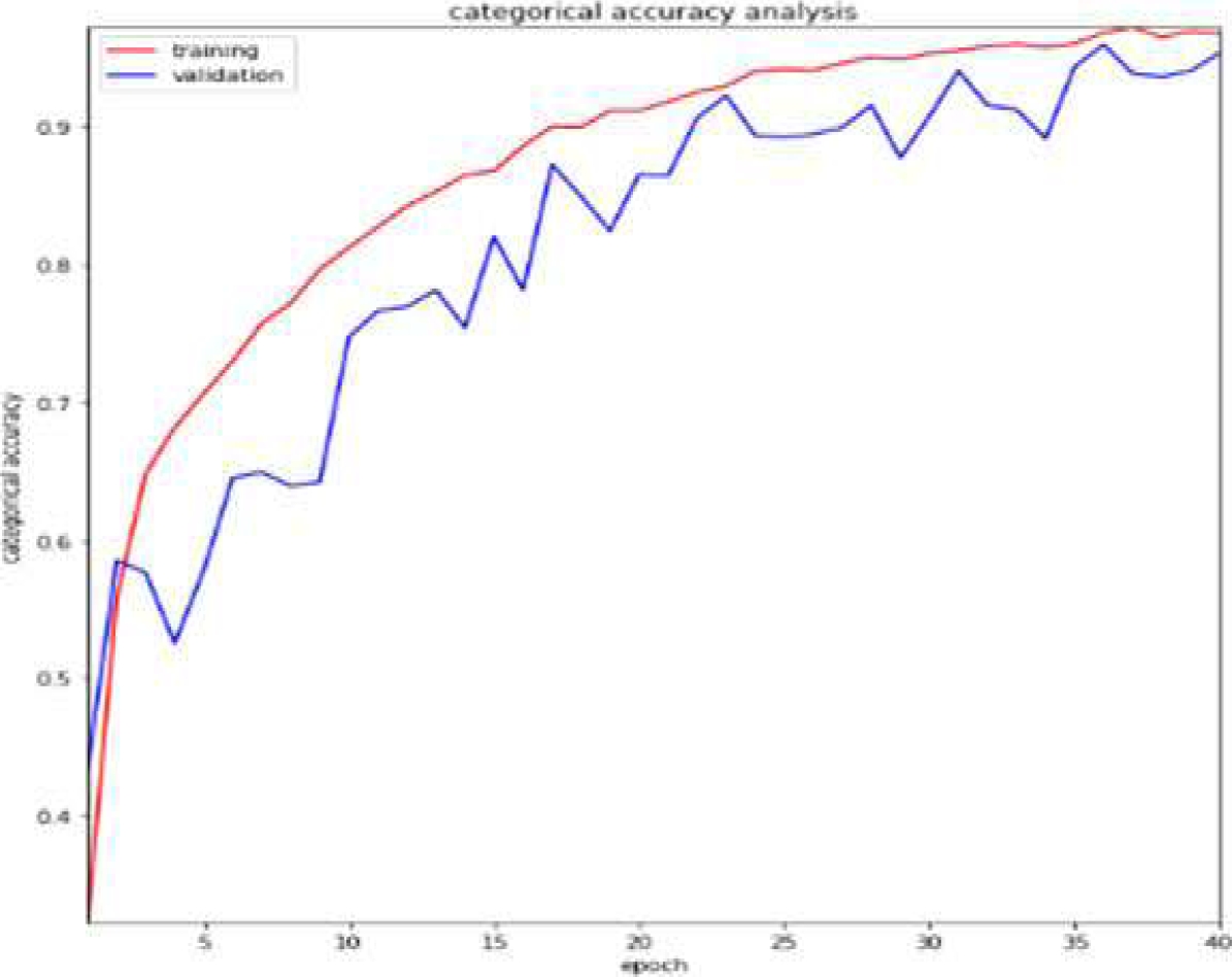
From Table 1, we get the classification performance of CANN, and Fig. 4 shows the accuracy plot.
Table 1 Classification performance of CANN
| Methods | AUC | Precision | Loss | Accuracy |
| CANN | 99.8% | 98.92% | 8.7% | 99.42% |

5 Comparative Study
There are several feature extraction techniques like PCA, ICA, and CANN, which are part of the dimensionality reduction process to create a manageable group to ease the process. These techniques can help to reduce the amount of big data for a better and more accurate model. From table 2, we get the comparison performance of PCA, ICA, and CANN.
Table 2 Comparison performance of PCA, ICA, and CANN
| PCA | ICA | CANN |
| The algorithm is used against data that is not labeled. It automatically split the dataset into groups based on their similarities. | Independent component analysis is one of the most frequently used dimensionality reduction techniques and is based on information theory. PCA searches for independent functions, which is the main distinction between it and ICA. | By changing the connected layer with the convolutional layer, the simple autoencoder structure changes to the convolutional autoencoder technique. |
Similar to PCA (principal component analysis) AEs perform dimensionality reduction in the compression phase. PCA is used for linear transformation and AE for nonlinear transformation.
5.1 ICA
The proposed ICA method is based on some criteria, which are defined by the FastICA algorithm [8]. It is possible to reconstruct an MRI picture using a linear combination of both the basic function and the corresponding coefficient. All MRI data are divided into testing and training datasets with an 8:2 ratio to get the best accuracy with comparable classified into different categories AD, MCI, and CN using SoftMax classifier. Our main motive for using ICA is to separate the observed signal from noise signals.
Here the two unsupervised techniques ICA and CANN are very useful among other related work to classify MRI images to distinguish MCI, AD, and CN subjects. For early diagnosis of Alzheimer’s disease, both ICA and CANN are very efficient biomedical techniques.
Therefore, in our research work, we want to give some light on biomedical applications to extract useful features by deleting unnecessary noise. ROI is one of the oldest techniques for analyzing Brain scans and is a very time and manpower-consuming process. Fig. 5, shows the architecture of ICA feature learning with proper steps for varieties of ICA techniques applied to separate the data.

Separate AD-related information or signal from noisy signals through ICA gives us a way to further research. For biomedical multi-subject data processing, human error is one of the important drawbacks for feature extraction of any type of disease. As a result, ICA is used for better feature extraction techniques for a more accurate diagnosis.
The extracted feature is fed into machine learning algorithm for classification. CA combined with SVM can make a better model for classifying different stages of Alzheimer's diseases into AD, MCI, and CN. FastICA features extracted with an SVM classifier had a 94.12 percent accuracy rate.
By using hybrid enhanced independent component analysis Basheera et al. analyzed MRI grey matter images with 90.4% [9]. ICA is a very powerful unsupervised technique for analyzing high-dimensional data.
To effectively distinguish between different stages of Alzheimer's, the mathematical model of ICA makes a difference in our research.
From Table 3, we get the Classification performance of Independent component analysis (ICA), and Fig. 6 shows the accuracy plot.
Combining ICA with SVM, we effectively analyzed and classify between different stages of disease into Alzheimer’s disease (AD), mild cognitive impairment (MCI), and cognitively normal (CN). Some of the biomedical techniques are not very suitable for the early diagnosis of disease.
A key challenge to address this problem is different unsupervised techniques to acquire focused based research on early detection of finding of AD.
ICA is among the unsupervised techniques used for feature extraction is also been effective in the case of Alzheimer's diagnosis with high accuracy. Similar techniques can be used for applications in brain imaging and health.
Working with data preprocessed with the ICA-model, artificial neural networks and support vector machines (SVMs) successfully extracted features using FastICA, and then trained SVM-based classifiers to discriminate AD, MCI, and CN separately with an accuracy of 94.12%.
Furthermore, it could be better research performance with machine learning technique for multiclass classification with 40 epochs.
The most notable variance we noticed was a 94.12% accuracy rate using T1 weighted MRI imaging of AD, MCI, and CN. Furthermore, we analyzed more models to process T2 weighted MRI images with other deep learning techniques for better performance.
6 Experiment and Result
6.1 Dataset
The dataset used for our model is taken from the ADNI database. For more detail, please go through the ADNI website. ADNI launches in 2003 as a partnership of both public and private to investigate diseases like Alzheimer in this study.
Researchers collect data different from this website for better research with study resources. Alzheimer's Disease Neuroimaging Initiative (ADNI) improves better clinical trials with a standardized protocol for the prevention and treatment of AD. ADNI has made a global impact for better diagnosis in the medical field. ADNI1 and ADNI2 are two participants who had 3.0 T T1-weighted images.
All images are downloaded in neuroimaging informatics technology initiative (Nifti) file format.
For diagnosed MRI analysis with CNN, procedures were performed on an Intel Xeor silver 4110 -2.1GHZ -3.5 GHz x8 core high-performance computer (HPC). We used the GPU platform, which has the largest collection of ALU cores with model Nvidia GTX1080Ti pascal chipset. Cuda(x) is stored in GPU (Graphics Processing Unit), where lots of external libraries are there and it has a channel where an organization creates its channel.
A collection of brain images was collected and proposed CANN and ICA with various classifiers were taken into consideration. fMRI and MRI are two techniques that are widely used to convey and provide anatomical information and are ideally suited for brain analysis research.
An unlabeled data for unsupervised training. The 64x64 patches are captured randomly from AD MRI data. convolutional autoencoder (CANN) consists of 6 layers in the structure. It has 4 groups of connections between different layers of CNN, i.e., convolutional layer, pooling layer, and fully connected layer.
Input: Input: 64×64 patch captured from MRI image. Different patches are collected from MRI slides.
C1: kernel is 5 × 5, in the first step, the number of convolution kernels is 50, and the non-linear function is Relu.
P1: max pool and size of pooling are 2 × 2.
C2: kernel is 5 × 5, in the first step, the number of convolution kernels is 50, and the non-linear function is Relu.
P2: max pool and size of pooling are 2 × 2.
C3: convolution kernel is 3×3 in the first step the number of convolution kernels is 50, and the non-linear function is Relu.
P3: max pool and size of pooling are 2 × 2.
Full: fully connected layer.
Output: SoftMax classifier, for 2 classes.
7 Classification
We compare the classification performance among CNN and ICA with unlabeled unsupervised learning in this result we classify to achieve the best accuracy with the lowest error rate in analyzing AD data. Fig. 7 shows the different stages of Alzheimer's disease by using the Keras library.

We employed three distinct architectures to represent similarity and classification as accuracy, precision, recall, and other metrics to conduct a full comparison in the table in Table 4.
Table 4 Classification performance of different CNN architecture
| CNN Architecture | Accuracy | Precision | Recall |
| VGG-16 | 99.43 | 98.92 | 98.01 |
| ResNet-50 | 92.43 | 92.13 | 93 |
| AlexNet | 93.13 | 92.12 | 93.11 |
As can be observed in Fig. 8, the accuracy is high and is approximately 99.42 percent.

8 Discussion
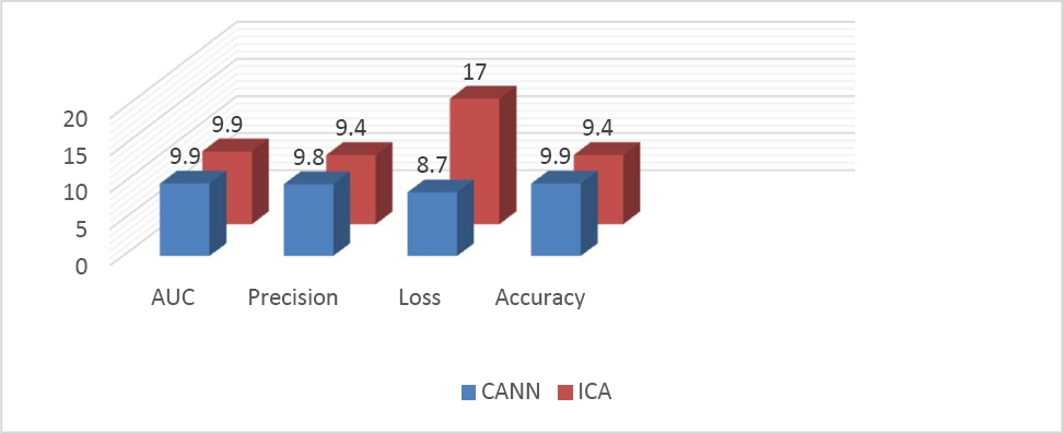
For a more accurate multiclass classification of Alzheimer's disease, with multiple stages measured through diverse research. We compared the two techniques and concluded that CANN is more applicable compared to ICA due to higher accuracy.
Deep learning approaches are a more satisfactory technique for showing an affordable result in critical studies.
Importantly, our algorithm performed well for varieties of high-dimensional datasets with better performance.
Although it was difficult to interpret heterogeneous MRI and fMRI data using multiple protocols, we found in our study that the examined model is not significantly affected by image value. To achieve high accuracy for dataset-specific approaches when categorizing AD or MCI, or CN patients, CNN was trained, validated, and evaluated in our studies utilizing high-dimensional datasets and various autoencoder techniques.
In conclusion, Fig. 8 shows the potential of performance to structure a model for early detection of AD.
9 Conclusion
In our research, High dimensionality is one of the key difficulties to manage huge medical data. Therefore, here is a detailed preview of one of the features of V's big data analytics characteristics. We examined the effects of two approaches, convolutional autoencoder (CANN) and independent component analysis (ICA), and found that CANN beats ICA models in terms of convergence speed and has a higher accuracy of 99.42%.
We also increase the precision of deep learning techniques for classifying various forms of Alzheimer's disease. We also wish to investigate how the impact manifests itself in other deep learning architectural methodologies with an effective approach to Alzheimer's disease.
Additionally, there is a good chance that the suggested method will be applied to other medical fields.

