


 nueva página del texto (beta)
 Inglés (pdf)
 Artículo en XML
 Referencias del artículo
 Enviar artículo por email
 Citado por SciELO
  Similares en
SciELO
Similares en
SciELO 
 Permalink
1 Introduction
Tropical cyclones (TCs) are weather-rotating systems that form associated with thunderstorms. These systems are characterized by a low-pressure center and extreme wind velocities [1, 2]. They go through four stages, from lower to higher intensity: tropical disturbance, tropical depression, tropical storm, and hurricane. TCs originate over tropical or subtropical ocean regions with sea surface temperatures (SSTs) around 27 °C.
These weather systems can cause deaths and considerable damage over coastal areas [3, 4, 5]. When TCs occur near the coast, like TC Bud, they can indirectly impact over distant inland areas. When they occur adjacent to the continent, convective storms develop over distant inland areas. According to [6], in the tropical Americas, a single TC can cause intense precipitation over inland arid regions.
Therefore, it is of fundamental importance to track down TCs well ahead to minimize societal damage and economic impacts. In general, numerical weather prediction (NWP) models, that run over supercomputers, are used to forecast the paths and strengths of TCs. The latter are highly interrelated with other atmospheric phenomena and strongly dependent on the variations of the SST, which depends on ocean feedbacks between the atmosphere and the ocean mixing layer.
NWP models use initial and boundary conditions to solve atmospheric dynamic and thermodynamic systems of partial differential equations with the assumptions of some semi-empirical physical approximations, known as parameterizations or parameterization schemes. The latter are linked with sub-grid scale processes that cannot be resolved explicitly by the governing equations implemented in the computer models.
The simulation of TCs with NWP models is very sensitive to the parameterizations used during the model runs. Several studies on the impact of parameterization schemes, when simulating mesoscale weather events, can be found in the literature.
It has been established that not only the physics options [7] but also the initial and boundary conditions in the initialization of NWP models [8, 9, 10, 11] play a decisive role in weather simulations. NWP models are currently used for both research and operational forecasting by different research and weather forecasting agencies around the world.
A sensitivity study is the most adequate to quantify the effect of different physics options; and, in turn, to predict the track path of a TC and its strength over a determined geographical region. Previous studies have made an effort to identify the optimum parameterization schemes and customize NWP models for the simulation and forecast of TCs over specific regions of the world.
For example, [12] documented a comprehensive assessment of the performance of parameterization schemes for TC computer simulations.
[13] performed a sensitivity study of the physics parameterizations when simulating the TC Jal over the Indian Ocean.
[14] performed sensitivity studies to evaluate cumulus parameterization schemes.
[15] conducted several sensitivity experiments for five TCs over the Bay of Bengal and found that the combination of the Kain-Fritsch for convection, the Yonsei University planetary boundary layer (PBL), the LIN for microphysics, and the NOAH for land surface schemes had the best performance to reproduce both the tracks and intensities.
Additionally, data assimilation has also been applied to provide data observations during the running of computer simulations to nudge the development of TC track paths, being considered a successful approach for improving TC forecasts [16, 17, 18]. However, this technique does not let the physical processes to evolve naturally. Besides, data assimilation techniques are very expensive, and they are not suitable to be implemented for forecasting purposes due to the high demand of computer resources.
In contrast to previous studies, we allowed the SST to evolve with the modeled atmosphere, for each model configuration, via the evolution of the computer simulations. According to the ocean temperature feedback between the modeled atmosphere and the ocean mixing layer, the purpose is to get reliable performance when the SST changes are taken into account in the development of TC Bud.
In this article, two ensembles of simulations with various parameterization schemes were carried out to define its members, from 00:00 UTC 10 June to 00:00 UTC 16 June 2018. A sensitivity study for a set of cumulus and microphysics parameterizations schemes was conducted to evaluate the track path and intensity of TC Bud. Three microphysics schemes, three cumulus schemes, and a moisture-advection-based trigger scheme were assessed. In one ensemble, the SST was fixed during the simulation period, while in the other one it was allowed to evolve with the modeled atmosphere via the computer simulations. The latter ensemble showed the best results.
The Weather Research and Forecasting (WRF-ARW) model was used with a new hybrid terrain-following sigma-pressure vertical coordinate. A parent domain and two child nested domains were established to define the grids over which the governing equations are solved. In the innermost domain, the assessment was performed with a grid spacing of 2 km.
This article is organized as follows. Section 2 describes the case study. Section 3 describes the model setup and methodology. Section 4 presents the results. Finally, in section 5, the conclusion is presented.
2 Case Study
TC Bud indirectly impacted the Mexican continental territory; when it occurred over the Eastern Pacific Ocean, heavy precipitation and flooding were present over inland Mexico. In Fig. 1a, the satellite spatial distribution of precipitation is observed. Fig. 1a was obtained and produced with the Giovanni online data system, developed and maintained by the NASA GES DISC.

Fig. 1 (a) Spatial distribution of observed averaged precipitation by satellite, at 02:00 UTC, on 12 June, produced with the Giovanni online data system, developed and maintained by the NASA GES DISC. (b) TC Bud’s best track (in black) and (in red) the track from the Global Forecasting System (GFS)
This TC occurred from 18:00 UTC 9 June to 06:00 UTC 16 June 2018, adjacent to the Mexican coastline, over the Eastern Pacific Ocean. In Fig. 1b, the best track (in black) is shown. Also, in Fig. 1b, the track obtained from the Global Forecast System (GFS) (in red) is also shown. The precursor of the TC was an easterly wave that emerged off the west coast of Africa on 29 May 2018 then entered the eastern North Pacific Ocean on 6 June. Later, a low pressure formed on 9 June, and it started to rotate.
Consequently, a tropical depression, 528 km south of Acapulco Guerrero, formed at 18:00 UTC. It became a tropical storm on 10 June at 00:00 UTC, reaching hurricane status on 10 June at 18:00 UTC. The maximum wind speeds reached 61.7 m/s at 00:00 UTC on 12 June near Manzanillo. Later, Bud became a tropical storm on 13 June at noon UTC, landfalling over Baja California Sur on 15 June at 02:00 UTC, with wind speeds of 20.5 m/s and a central pressure of 999 hPa. Subsequently, it crossed Baja California Sur, weakening due to the interaction with land.
The TC converted into a convection-free post-tropical cyclone on 15 June at noon UTC, and the isobaric contours opened by 00:00 UTC on 16. Then Bud dissipated by 06:00 UTC on 16 June. In Fig. 2, a representation of part of the evolution of the TC Bud is shown. In this figure, the maximum wind speed (MWS) and the sea level pressure (SLP), obtained from one computer simulation, are shown.

3 Modeling Setup and Methodology
The (WRF-ARW) model, version 4.1.3 [19], was used to simulate TC Bud. The model has a fully compressible and non-hydrostatic dynamic core. It allows to simulate and forecast mesoscale convective systems with many parameterization schemes. This mesoscale numerical model was developed for research and operational forecasting. The WRF-ARW model was implemented in the CÓDICE B2 cluster at Centro de Investigación en Computación (CIC) of the Instituto Politécnico Nacional (IPN), using 16 nodes. Each node has 28 CPU cores.
In each of the two ensembles, the outer domain was set with a grid spacing of 18 km, while the innermost domain with a grid spacing of 2 km, using a ratio of 1 to 3 and two-way nesting.
In order to assess the different cumulus and microphysics parameterizations at 2 km grid spacing (over the innermost domain, d03, shown in Fig. 3), the initial and boundary conditions (IBCs) were downscaled. In Fig. 3, the nested domains d01, d02, and d03 with 18, 6, and 2 km grid spacing, respectively, are shown.

Fig. 3 Domain setup for the study. The assessment was carried over the innermost domain, d03, with a grid spacing of 2 km
The IBCs were obtained from the National Center for Environmental Prediction (NCEP) FNL operational global analysis and forecast dataset, which is available with a grid spacing of 0.25° at 6 h intervals.
In this dataset, the files that contain the IBCs are made with the same model used in the Global Forecast System (GFS). To obtain more inputs, the data was interpolated at intervals of 3 h and used to update the outermost domain during each simulation, every 3 h. The innermost domain, covering the MTC region and the adjacent Pacific Ocean, is comprehended by a horizontal grid of 886 × 886 points. The model was configured with 51 vertical levels, using the new hybrid sigma-pressure vertical coordinate that follows the terrain and gradually makes the transition to constant pressure surfaces, reducing the numerical noise at higher levels [20, 21].
A 3 s time-step for the innermost domain was selected via the evolution of the simulations. A time-step ratio of three was chosen for the middle and outermost domains. In comparison to greater time-steps, a short time-step ensures a better simulation performance in terms of satisfying the Courant-Friedrich-Lewy condition [22]. The model needed to be warmed up (spin up) 17 h before analysis since simulation results are sensitive to the spin-up time [23].
Three different microphysics and cumulus schemes, with and without convection triggering, were varied one at a time–while the other schemes were left unchanged in each ensemble. The microphysics schemes used were the Purdue Lin scheme [24], the WRF single-moment 6-class scheme [25], and the Thompson scheme [26]. The cumulus schemes used were the Kain-Fritsch scheme [27], the Betts-Miller-Janjic scheme [28], and the simplified Arakawa-Schubert scheme [29]. The unchanged schemes were the Yonsei University scheme [30] for the planetary boundary layer, the MM5 similarity scheme [31, 32, 33, 34, 35] for the surface layer, the unified Noah land surface model [36] for the land surface, the Dudhia shortwave scheme [37] for the shortwave radiation, and the RRTM Longwave scheme [38] for the longwave radiation. A moisture advection-based trigger scheme was also considered.
In the first ensemble, the SST was provided, from the Real-time Global Sea Surface Temperature Analysis product (RTG-SST), for the period simulated over the ocean surface. In the second ensemble, just the IBCs from NCEP FNL were used, and the names for each ensemble member will end in “-GFS.” Each ensemble member of the first ensemble, which performed better than the second, is listed in Table 1. During the numerical simulations, the SST was modified according to the response of the surface winds and changes in radiative fluxes using the scheme proposed by [39]. The change in SST on a daily scale is not considerable; however, subtle changes could indirectly impact the simulated atmosphere. During TCs, surface winds cause ocean mixing over the first few meters, changing the SSTs. According to [40], negative feedback from wind-driven ocean mixing can be reflected in numerical simulations.
Table 1 Ensemble members of the ensemble with RTG-SST forcing
| Simulation | Simulation acronym | Microphysics parameterization | Cumulus parameterization | |
| 1 | LIN-KF-RTG | Purdue Lin scheme | Kain-Fritsch scheme | |
| 2 | LIN-BMJ-RTG | Purdue Lin scheme | Betts-Miller-Janjic scheme | |
| 3 | LIN-SAS-RTG | Purdue Lin scheme | Simplified Arakawa-Schubert Scheme | |
| 4 | LIN-KF-TR-RTG | Purdue Lin scheme | Kain-Fritsch scheme | Moisture advection-based trigger scheme |
| 5 | THOM-KF-RTG | Thompson scheme | Kain-Fritsch scheme | |
| 6 | THOM-BMJ-RTG | Thompson scheme | Betts-Miller-Janjic scheme | |
| 7 | THOM-SAS-RTG | Thompson scheme | Simplified Arakawa-Schubert scheme | |
| 8 | THOM-KF-TR-RTG | Thompson scheme | Kain-Fritsch scheme | Moisture advection-based trigger scheme |
| 9 | WSM6-KF-RTG | WRF Single-moment 6-class scheme | Kain-Fritsch scheme | |
| 10 | WSM6-BMJ-RTG | WRF Single-moment 6-class scheme | Betts-Miller-Janjic scheme | |
| 11 | WSM6-SAS-RTG | WRF Single-moment 6-class scheme | Simplified Arakawa-Schubert scheme | |
| 12 | WSM6-KF-TR-RTG | WRF Single-moment 6-class scheme | Kain-Fritsch scheme | Moisture advection-based trigger scheme |
4 Results
Both cumulus and microphysics schemes play an important role when forecasting TCs. Cumulus schemes are associated with redistribution of moisture and heat, in the vertical direction, but they do not depend on the latent heat generated during condensation and deposition of water vapor. Besides, latent heat is important in the vertical development of convection inside TCs. During lifting, latent heat is released due to condensation or deposition. On the other hand, microphysics schemes depend on the moisture distribution in the troposphere, where heat transfer occurs between the ocean surface and the uppermost layers of the atmosphere.
The simulated tracks with and without SST forcing were compared with the best track data. The simulated paths closer to the best track path are those obtained from the ensemble members with SST forcing, which are discussed in this section. However, in Table 2, the mean track error for the ensemble members without SST forcing is shown. The tracking error was calculated as the distance between a point in the simulated track path and a point in the best track path along the corresponding great circle for all the ensemble members. Then, the average track error for each track was obtained.
Table 2 Mean track error (in km): ensembles without SST forcing
| LIN-KF-GFS | 110.062 |
| LIN-BMJ-GFS | 83.624 |
| LIN-SAS-GFS | 44.6 |
| LIN-KF-TR-GFS | 44.551 |
| THOM-KF-GFS | 64.651 |
| THOM-BMJ-GFS | 95.147 |
| THOM-KF-TR-GFS | 35.337 |
| THOM-SAS-GFS | 46.612 |
| WSM6-KF-GFS | 79.583 |
| WSM6-BMJ-GFS | 76.741 |
| WSM6-SAS-GFS | 56.172 |
| WSM6-KF-TR-GFS | 34.471 |
Fig. 4a provides the simulated track paths for the WSM6-KF-RTG (with SST forcing) and WSM6-KF-GFS (without SST forcing) of TC

Fig. 4 (a) Track paths with longitude (deg) and latitude (deg) coordinates for WSM6-KF-RTG (with SST forcing) and WSM6-KF-GFS (without SST forcing) ensemble members. (b) Sea Level Pressure (SLP) for the THOM-KF-GFS, WSM6-KF-GFS, and LIN-KF-GFS ensemble members (without SST forcing). Best track observations are also included; as well as the track from the Global Forecasting System (GFS) in (a), shown in red The simulated track paths, the SLP along the tracks, and the MWS for the different cumulus and microphysics schemes, for the ensemble with SST forcing are presented from Fig. 5 to Fig. 7. Although the computer simulations can reproduce the best track path, they are not capable enough to predict the MWS
Bud. It is observed that the ensemble member with SST forcing is closer to the best track path than the one without SST forcing. Besides, in Fig. 4b, the SLP for each of the THOM-KF-GFS, WSM6-KF-GFS, and LIN-KF-GFS ensemble members, along with the best track SLP (in black), is shown. The SST was not allowed to evolve with the modeled atmosphere with the Kain-Fritsch cumulus parameterization in the latter ensemble members.
It is noticed that the mentioned ensemble members overestimated the SLP of the TC. The same occurred for all other ensemble members of the ensemble without SST forcing. However, the simulated SLP improves when SST is allowed to evolve with the modeled atmosphere for most ensemble members with SST forcing.
This can be appreciated in Fig. 5b when the SLP improves compared to Fig. 4b.

Fig. 5 (a) Track paths with longitude (deg) and latitude (deg) coordinates for THOM-KF-RTG, WSM6-KF-RTG, and LIN-KF-RTG (with SST forcing) ensemble members. (b) Sea Level Pressure (SLP) for each of the ensemble members in (a). (c) Wind Speed, the maximum values of TC Bud (MWS), for each of the ensemble members in (a). Best track observations are also included; as well as the track from the Global Forecasting System (GFS) in (a), shown in red
The simulated track paths, the SLP along the tracks, and the MWS for the different cumulus and microphysics schemes, for the ensemble with SST forcing are presented from Fig. 5 to Fig. 7. Although the computer simulations can reproduce the best track path, they are not capable enough to predict the MWS. The mean track errors for the THOM-KF-RTG and the WSM6-KF-RTG ensemble members, shown in Table 3, when the Kain-Fritsch cumulus scheme is used, are lower than the mean track error for the LIN-KF-RTG ensemble member. This is appreciated in the track paths shown in Fig. 5a. However, in the first hours of simulation, the track from THOM-KF-RTG considerably departs from the best track, but it presents the lowest mean track error along with the whole TC event.

Fig. 6 As in Fig. 5, but for THOM-KF-TR-RTG, WSM6-KF-TR-RTG, and LIN-KF-TR-RTG ensemble members, see Table 1 for acronyms

Fig. 7 As in Fig. 5, but for THOM-BMJ-RTG, WSM6-BMJ-RTG, and LIN-BMJ-RTG ensemble members, see Table 1 for acronyms
Table 3 Mean track error (in km) taking into account SST forcing
| THOM-KF-RTG | 47.002 |
| WSM6-KF-RTG | 47.031 |
| LIN-KF-RTG | 70.041 |
In Table 4, the mean track error for the THOM-KF-TR-RTG, WSM6-KF-TR-RTG, and LIN-KF-TR-RTG ensemble members are shown. These ensemble members consider a moisture-advection-based trigger scheme for the Kain-Fritsch cumulus scheme. The latter considerably improved the mean track error for the three microphysics schemes.
Table 4 Mean track error (km) taking into account SST forcing
| THOM-KF-TR-RTG | 32.207 |
| WSM6-KF-TR-RTG | 26.314 |
| LIN-KF-TR-RTG | 39.551 |
In these three ensemble members, with three different microphysics schemes, the THOM-KF-TR-RTG was the one that performed best, appreciated in Fig. 6a. However, the LIN-KF-TR-RTG is the ensemble member that best describes pressure reduction; see Fig. 6b. The THOM-KF-TR-RTG and LIN-KF-TR-RTG ensemble members qualitatively describe wind speed increase, although they do not reach the maximum value of the best track data for this variable.
Microphysics schemes that depend on cumulus schemes at coarse grid spacing domains are important in regional weather models for providing atmospheric heat and moisture tendencies [41].
Vertical flux of cloud, precipitation, and sedimentation processes of hydrometeors are also included in the microphysics schemes. The microphysics schemes used, as aforementioned, were the Purdue Lin, the WRF single moment 6-class, and the Thompson scheme.
The first includes cloud water, cloud ice, non-precipitable water, rain snow, and graupel [24]. In the second scheme, the ice crystal number concentration is expressed as a function of the ice amount [25]. Finally, the Thompson scheme is a 6-class microphysics scheme with graupel, ice, and rain number. It includes a generalized gamma distribution for each hydrometeor species with snow parameterization, depending on the ice water content and the temperature.
When the Betts-Miller-Janjic cumulus scheme was used in the computer simulations, the mean track errors, when compared to the best track data, were worse than the previous results. In Table 5, the mean track error for each ensemble member with this cumulus scheme is shown.
Table 5 Mean track error (km) taking into account SST forcing
| THOM-BMJ-RTG | 85.028 |
| WSM6-BMJ-RTG | 68.875 |
| LIN-BMJ-RTG | 78.262 |
The simulated MWSs was underestimated by all the different combinations that defined each ensemble member. The SLP did not exactly reproduce the pressure evolution from the best track information, but this variable described the observed minimum for each ensemble members with SST forcing. The mean SLP for the ensemble members with the Simplified Arakawa-Schubert cumulus scheme is presented in Fig. 8b.
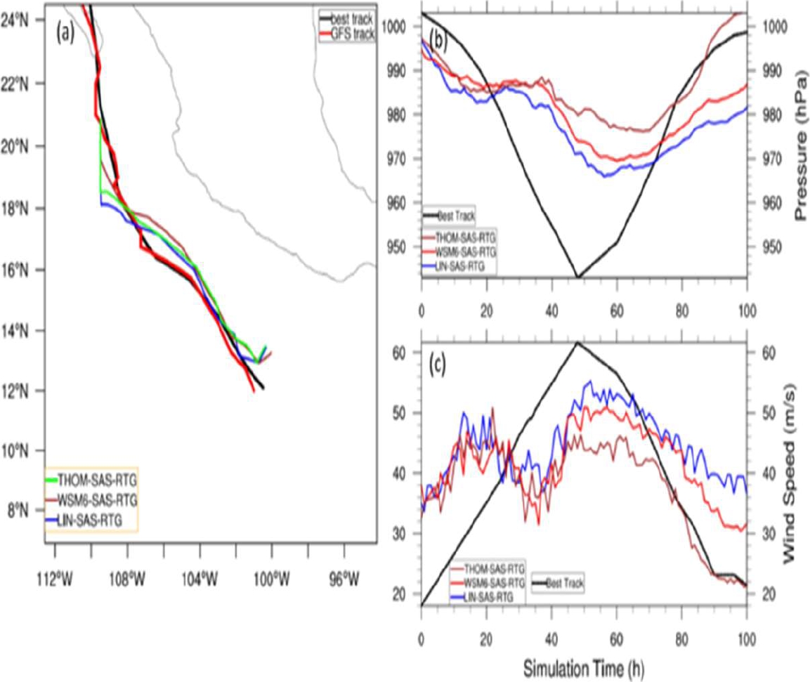
Fig. 8 As in Fig. 5, but for THOM-SAS-RTG, WSM6-SAS-RTG, and LIN-SAS-RTG ensemble members, see Table 1 for acronyms
The evolution of MWS for each ensemble member is shown in Fig. 8c. The mean track errors for the THOM-SAS-RTG and the LIN-SAS-RTG ensemble members did not improve, showing greater values than those without SST forcing, presented in Table 6.
5 Conclusion
The simulation of TC Bud using the WRF-ARW model, using the cluster CÓDICE B2, is documented by studying the sensitivity of different cumulus and microphysics schemes. This event was selected because TC Bud reached category-4 hurricane status, spending its lifespan over the Eastern Pacific Ocean and dissipating over the Gulf of California without traversing Mexico. Based on our experimental results, we summarize the following findings:
Overall, the computer simulations have performed well in predicting the track path of the TC.
Nonetheless, in any case, regardless of the cumulus and the microphysics schemes, the simulations underestimated the strength (expressed by either the SLP or the MWS) of the cyclone.
The best ensemble members were those in which the moisture-advection-based trigger scheme, with the Kain-Fritsch cumulus scheme, was used, regardless of the microphysics schemes. This was reflected in the obtained best mean track error values.
The track paths calculated from the THOM-SAS-RTG and the LIN-SAS-RTG ensemble members did not show an improvement compared to those that did not include SST forcing.

