


 nueva página del texto (beta)
 Inglés (pdf)
 Artículo en XML
 Referencias del artículo
 Enviar artículo por email
 Citado por SciELO
  Similares en
SciELO
Similares en
SciELO 
 Permalink
1 Introduction
Heart noises are the expression of the opening and closing of the four cardiac valves, where the muscular contraction that drives the blood from one cavity to another generates a high acceleration and delay of the blood flow causing a pressure differential [12, 15]. Its normal physiological functioning is unidirectional, which allows the correct circulation of blood through the cardiovascular circuit. However, abnormal noises can be produced when the heart valves do not close or open completely, causing leaking backwards and the interruption of laminar blood flow by turning into a turbulent flow. These sounds are called murmurs, and their correct identification during auscultation, as part of the diagnosis procedure, is crucial to detect potentially life-threatening heart conditions.
Apart from traditional auscultation, these sounds can be recorded and digitized using electronic stethoscopes, which generate phonocardiographic (PCG) signals. The identification of abnormalities of the mechanical functioning of the heart is based on a series of features extracted from the PCG recordings, where computer-aided analysis allows to identify between normal and abnormal records, since these vary among themselves with respect to their temporal and spectral characteristics.
Therefore, the precise feature extraction is key for a correct classification of heart sounds and can play an important role in assisting the medical community in speeding up and improving the diagnosis.
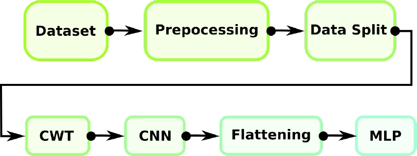
This article addresses the problem of identifying abnormal heart conditions using features from the PCG recording in both time and spectral domain, extracted through a technique known as Continuous Wavelet Transform, and a based Deep Learning (DL) methodology known as Convolutional Neural Networks (CNN). The output of the network grants the probability that a particular PCG recording belongs to a normal or abnormal class. The summary of the proposed model as a block diagram is shown in Fig. 1.
2 Related Work
Several laboratories, using particular datasets, have approached the heart sounds classification problem using their own distinctive AI methodology [14]. However, to make a correct comparison, it is necessary to select those works that use the same database as in the present work. Table 1 summarizes the feature extraction techniques and classifiers used, along with the results respectively obtained, using the same open access dataset [17].
Table 1 Comparative table between works that used the same dataset
| Author | Feature Extraction | Classifier | Precision | Recall | Specificity | Global Accuracy |
| Son et al. 2018 [17] | DWT and MFCCs | SVM, KNN, DNN | – | 98.2% | 99.4% | 97.9% |
| Alqudah, A. M. 2019 [4] | Eight statistical moments from the Instantaneous Frequency Estimation + PCA | KNN* and Random Forest | 100% | 98.28% | 100% | 94.8% |
| Ghosh, S.K. et al. 2019 [7] | Wavelet Synchrosqueezing Transform | Random Forest | – | – | – | 95.13% |
| Upretee, P., and Yuksel, M. E. 2019 [18] | Centroid Frequency Estimation | SVM and KNN* | 99.6% | 99.76% | 98.83% | 96.5% |
| Ghosh, S.K. et al. 2020 [6] | Local energy and entropy from Chirplet Transform | WaveNet | 98.0% | 98.1% | 99.3% | 98.33% |
However, a point noted is the trifle with which they approach the training of their models. It is possible to observe in [17, 18, 13] that the reported results are those obtained during training since the number of the samples shown in the confusion matrices, sums as the total of samples in the dataset.
This has important implications for the interpretation of the reported results since through training it is only possible to know the memorization capacity of the classification algorithm and the degree of compaction of the data. It is not possible to evaluate an actual performance if it is not through a test data set that the classifier has never seen.
Furthermore, the use of Convolutional Neural Networks (CNN), along with the spectral decomposition known as Continuous Wavelet Transform (CWT), has never been used to classify heart valve disease, placing the present work as a new methodological proposal.
3 Materials and Methods
This section summarizes the feature extraction techniques and Deep Learning algorithm used to address the problem apropos the HVD detection, along with the dataset description. The algorithmic proposal was developed in Python 3.9 on the Ubuntu 20.04 distribution. In particular, the deep learning algorithm was built on Keras 2.4.3.
3.1 Dataset
The PCG signals used in this article were obtained from an open database [17]fn, containing 200 records for each of the following five classes:
— Aortic stenosis (AS).
— Mitral regurgitation (MR).
— Mitral stenosis (MS).
— Mitral valve prolapse (MVP).
— Normal (N).
Each signal was sampled at 8000 Hz, with durations of at least one second. To maintain uniformity in the data analysis, two windows of 6144 data points (0.768 s) were taken from each signal, each one containing at least one complete cardiac cycle, therefore, duplicating the number of samples from 200 to 400 for each class.
It is possible to notice that the Normal (N) and Pathological (AS, MR, MS, MV) classes, with a ratio of 4:1, are strongly unbalanced. This has implications for the model training, as mentioned in the previous section. Since the Normal class was separated into training and test subsets containing 320 (80%) and 80 (20%) time series, respectively, it was necessary to select the same subsets of the Pathological class to avoid the related bias. Therefore, 80 random samples of each subclass (AS, MR, MS, MVP) were selected to structure the other half of the training subset.
Afterward, each time series was transformed using CWT. The implications of using this extraction technique and the procedure are discussed forward.
3.2 Continuous Wavelet Transform
CWT is a spectral decomposition method which is based on representing the signal in the form of wavelets with different displacement and scaling factors, where the use of the correct mother wavelet (MW) drives the enhancement of the waveforms of interest.
The MW is an effectively limited waveform in duration, with an average equal to zero. The MW used in the CWT was a Morlet, described by:
And starting with an MW
where
Thus, the CWT of a signal
where the integral is solved for
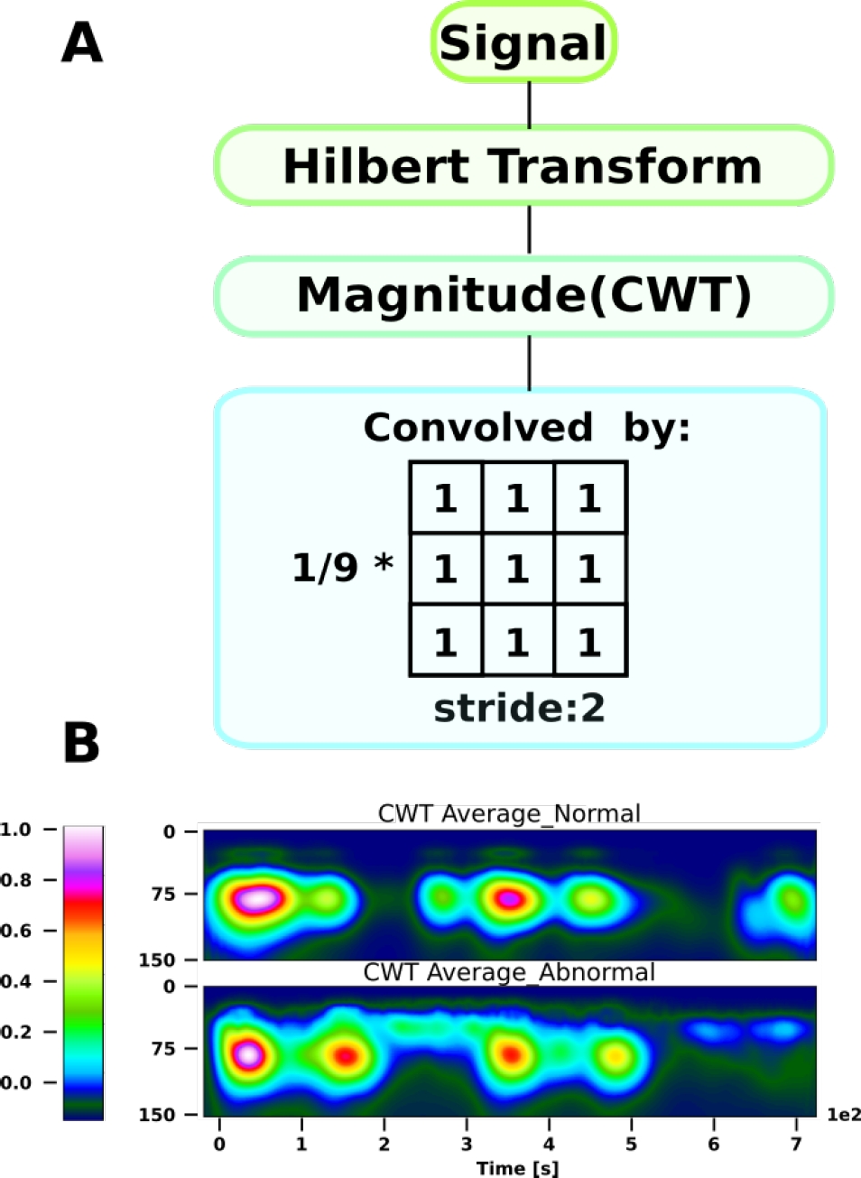
However, as a previous step to the CWT calculation, the Hilbert transform was implemented since this transform is an efficient tool to extract the time-localized amplitude and phase of a mono-component signal, with scale and translation invariance, and its energy-conserving (unitary) nature [5, 11]. The Hilbert transform
It is possible to observe that this gives us a complex representation. To retrieve all the information of the signal, it is necessary to select a complex MW such as Morlet. By applying the CWT, we obtain a matrix representation of the coefficients of size
3.3 Convolutional Neural Network (CNN)
Deep learning refers to AI models capable of extracting features, with multiple levels of abstraction and learning representations of data, without the need for a human expert agent that transformed the raw data into suitable internal features from which the learning subsystem, could detect or classify patterns in the input [8].
In particular, CNN discovers intricate patterns in datasets by using the backpropagation to optimize how a set of filters need to change their internal parameters to compute the attributes that best represent the data in a highly compact depiction [10].
The proposition of the decomposition into a spectral space through CWT may be counterintuitive. However, since CNN uses filters that look for local spatial patterns (the locality depends on the size of the filter), the frequency dynamics of the PCG records over time contain richer information than the simple temporal dynamics of the time series.
As it is possible to see in the flow chart shown in Fig. 3, the CNN introduces a special network structure, which consists of the so-called convolution and grouping layers alternately that allow extracting the main characteristics of the coefficient matrices [1].

Fig. 3 Block diagram of the complete process: Dataset pre-processing and splitting, feature extraction, classification using a deep neural network
When using CNN for pattern recognition in phonocardiographic sounds, the input data must be organized as a series of feature maps. Since CWT was used to find spectral coefficients along time, the expected input structure for a 2D CNN occurred naturally, where each of the coefficients represents the pixel values.
Once the input feature maps are formed, the convolution and grouping layers apply their respective operations to generate the activation of the units in those layers, in sequence. The discrete convolution between the filter and the coefficient matrix is mathematically defined as:
It is possible to deduce that, if the image dimension is given by
Max-pooling is a particular case of a convolutional layer, where the filter is a matrix of ones and, after the convolution, a maximum function is applied. By convention, we consider a square filter with dimensions
In CNN terminology, the pair of convolution and max-pooling layers in succession is often referred to as a convolutional layer [3]. Each of these layers is in charge of finding, building attributes and reducing the dimensionality of the input matrix to a characteristic pattern.
Finally, this pattern is vectorized (flattened) and fed to a multilayer perceptron network (MLP), which will act as a classifier. In reality, nothing prevents the use of any other architecture or classification model, however by convention MLP is the most commonly used.
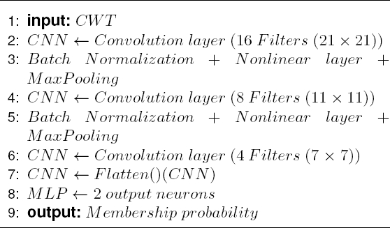
The proposed architecture of the CNN is described as pseudocode in the Algorithm 1.
3.4 Performance
The evaluation and validation of the machine learning algorithm is an essential part of any AI project. The model can give satisfactory results when it is evaluated using a metric, such as accuracy, but most of the time using a single metric is not enough to judge the performance of our model. That is why, in this section, the four evaluation metrics used are defined, where the primary building blocks are the true positive
Accuracy: It is the ratio between the number of correct predictions and the total number of input samples:
Due to its construction, this metric is not ideal when the classes are unbalanced (as is the case with the dataset used). The problem arises when the cost of misclassifying samples from minor classes is very high. If we are faced with a rare but fatal disease, the cost of not diagnosing a sick person’s illness is far greater than the cost of sending a healthy person for further tests. Therefore, it is necessary to use metrics based on relevance, that is, that do take into account the imbalance of the classes, such as precision and recall.
Precision and recall: Precision (also called positive predictive value) is the fraction of relevant instances among the retrieved instances:
While recall (also known as sensitivity) is the fraction of relevant instances that were retrieve:
Finally, since in a clinical test the goal is to accurately identify people who have a particular condition (where its misclassification into a non-pathological class could be fatal), the ratio between true negatives and false positives should be accounted for, giving rise to a metric known as specificity. In other words, specificity measures how the test is effective when used on negative individuals:
4 Results
During the construction of the model, the experimentation focused on two variables: the number of scales to be used in the CWT and the generation of the training subset, which as mentioned in section 3.1, is partially built from 320 pseudorandomly selected items from the Pathological (AS, MR, MS, MVP) subclasses.
For the case of CWT, the value of the power coefficients obtained for each scale at each time point, averaged for each of the class sets, with 150 scales is shown in Fig 2. The number of scales depends on the MW used to perform the decomposition, since each MW has a specific morphology and central frequency that will change as a function of scale. There is an approximate relationship between scale and frequency defined as:
where
On the other hand, to ensure that the CNN’s performance was since the optimum (local) minimum was found, which ensures the generalizability of the model, and not from the pseudo-random selection of the data, a 6-fold cross-validation method was applied, where the overall accuracy obtained was 97.70 ± .432.
By having an overall accuracy with a standard deviation of less than 0.5%, the proposed model execution can be attributed to its generalizability, which allows us to select the best of the runs of our classifier to evaluate its performance. Fig. 4B shows the detailed accuracy, precision, recall and specificity obtained using 20 % of the dataset as the test set. It is possible to observe that 98.2% of the classes were correctly classified according to the binary accuracy.

Fig. 4 DL performance results (20% of the dataset as the test set): A Confusion matrix used to calculate the metrics. B Precision, Recall, Specificity and Accuracy for the test dataset classification. The vertical axis shows only the percentage from 0.8 to 1.0 to facilitate the visualization of the results. ”N” and ”P” stand for Normal and Pathological class respectively
Furthermore, the confusion matrix, from where all the metric calculations were based, is shown in Figure 4A, where each column of the matrix represents the number of predictions of each class, while each row represents the instances in the real class.
5 Conclusion
This article focused on the classification of HVD from 1000 PCG records, combining a deep learning algorithm with time-frequency analysis wherein the time-series recognition problem is transformed into an image recognition problem. To do so, the spectral characteristics through time were extracted using CWT, and given the dimensional nature of these features, it was decided to use a CNN to classify each recording as Normal or Pathological, since this is the first step in the diagnostic procedure. If an abnormality is present, further clinical tests must be carried out to determine the type of abnormality. This approach has never been used, placing it as an innovative methodological proposal.
Furthermore, the model had a performance, measured through its accuracy, above 98.2%, surpassing four of the five models described in the literature (Table 1), placing it as a competitive and efficient model for the classification of valvular diseases.
In addition, one of the necessary metrics to measure competitiveness in clinical diagnostic systems, and where the present work takes into account and stands out, is specificity (section 3.4), obtaining 99.5%, which means that less than 1% of the Pathological PCG records will be classified as Normal.
This provides robustness to the model and invites to implement it in a system for the assisted diagnosis of heart valve diseases to improve the prognosis of patients, reducing the error associated with the experience of the medical crew.

