


 nueva página del texto (beta)
 Inglés (pdf)
 Artículo en XML
 Referencias del artículo
 Enviar artículo por email
 Citado por SciELO
  Similares en
SciELO
Similares en
SciELO 
 Permalink
1 Introduction
Traffic congestion on city roads has become a significant issue that must be addressed in urban development due to urbanization and the rapid rise in vehicles The acceleration of urbanization and the rapid increase within the number of vehicles for travel have made traffic congestion on urban roads a serious problem that must be addressed in urban development. As a result, several researchers suggested the concept of “carpooling”. Experimental results have shown that this idea demonstrates the effectiveness of policies in reducing urban traffic congestion.
In March 2013, researchers at the Massachusetts Institute of Technology (MIT) analyzed a week of taxis in Manhattan, New York [1]. Approximately 10,000 of New York’s 13,600 taxis were used during the hour. To meet its 98% transportation requirement, Manhattan only needs 3,000 shared taxis. This study found that an effective carpooling system reduces traffic congestion in cities and improves the speed of passenger transportation for in-service vehicles and drivers’ operating benefit.
Furthermore, energy consumption and environmental pollution should be reduced [9]. Accordingly, implementing carpooling is an effective way to increase the quality of urban traffic [10, 12]. Some cities have introduced and incorporated taxi ride sharing as a means of reducing taxi traffic congestion. As a result, carpooling has sparked the attention of many researchers as an intriguing subject of urban transportation science. In 2011, Agatz investigated the issue of driver and passenger assignment in a competitive environment and suggested a method for maximizing vehicle mileage and individual travel costs [2].
Shinde presented a multi-objective optimization-assisted carpool path matching genetic algorithm. The algorithm reduces computational complexity and time intervals while also improving the carpool effect [19]. In 2015, Pelzer proposed a dynamic decision algorithm that supported the partition of the network [19]. The algorithm divides and numbers the road network and uses the spatial route search algorithm for matching passengers and vehicles.
In 2015, Jiau used a genetic algorithm to implement carpool path matching in a short amount of time, resulting in a carpool path matching scheme with low complexity and memory [13].
In 2015, Huang suggested a fuzzy control genetics-based carpooling algorithm that combines a genetic algorithm and a fuzzy control system to optimize the route and balance driver assignments and demands in an intelligent carpooling system [11].
Cheng developed a multi-dynamic taxi ride sharing model in 2013, using the genetic algorithm to solve the carpool problem to benefit travelers and drivers [6].
In 2013, Ma proposed a large-scale carpooling service; it responds efficiently to real-time requests sent by taxi users and generates carpooling schedules that significantly reduce the total distance of the trip [15].
Xiao et al. developed a membership function based on three factors: driving directions, driving time, and the number of passengers in 2014 to achieve fuzzy carpool grouping and identification of passengers and taxis [23].
In 2017, Zhang proposed the first systematic work, named CallCab, based on a data-driven methodology to design a single recommendation system for daily and ride-sharing services. This recommendation system was designed to help passengers find the best taxi with carpooling [25].
As shown in Figure 1, which was generated by extracting requests from New York Taxi data over two separate periods, mobility requests develop over time, and the distribution of requests is uneven [20].
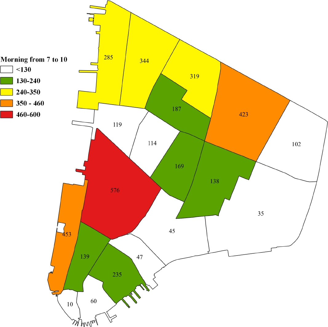
Fig. 1 Observed demand imbalance in NY Taxi dataset [20] trips between morning (7-10 am) and evening (6-9 pm) in the south part of Manhattan on Tuesday, July 7, 2016 (morning)
It can result in an unbalanced distribution of drivers for RS systems, as seen in ??, where the majority of demand is concentrated in the upper region, and most vehicles are located on the opposite side after their last journey, where fewer new customers request a ride [4].
2 Related Work
Taxi rebalancing can be categorized into approaches based on static zones [8, 7, 3, 22, 21] and dynamic zones [5, 14]. In the generation of static rebalance zones, the relocation zones’ geographic coverage is predefined at design time. For example, the New York Manhattan area is divided into predefined areas that do not change over time [8]. Each vehicle, using cross-learning, learns and decides at each time step whether to move to one of the neighboring areas or to stay in its current area. Austin’s rebalancing zones are established by dividing the city into 2 square mile square blocks in [7].
For each location, a block weight is calculated to account for the excess or deficit of vehicles in the block in the sense of expected travel supply and demand. The forecast travel demand is determined from historical data and current demand, and blocks with a low weight aim to collect vehicles from the community where there is a surplus. The zones were identified using a fine-grained grid but also static [3]. If a vehicle is idling, it will rebalance itself using its local knowledge: it determines whether or not to rebalance towards a neighboring region based on the distribution of demand in the surrounding areas [8]. According to the route of the road network, the works presented in [7] divide the region into rebalancing areas.
The zones are defined so that for each region Ri, a zone makes it possible to reach Ri in the time allotted. Idling vehicles are rebalanced to prevent excess vehicles in the same area, taking into account travel time to reduce empty journeys and potential demand, calculated from the current order. However, the zones do not adjust based on traffic conditions or the number of taxis once they have been established. The majority of approaches only allow rebalancing for idling cars. In contrast, rebalancing was combined with carpool assignment, allowing carpool pick-up from zones neighbors, reducing passenger waiting time but increasing travel time [3, 8].
A dynamic zone generation algorithm was used for balancing; rebalancing zones were calculated using a clustering algorithm. On the queries produced by a distribution specified on historical data, k-means clustering is applied [5].
Consequently, the coverage and size of the zones can change, but the total number of zones remains constant. the second approach uses EM clustering and allows to create a different number of zones according to different densities of requests[14]. Furthermore, the approach uses real-time data rather than historical data to better respond to dynamic demand.
Both approaches are similar to the current, in which a particle swarm optimization (PSO) clustering algorithm was used to generate dynamic zones for balancing unoccupied vehicles, with a fixed number of zones based on real-time data.
3 Background
This section presents the basic information needed to understand the design and implementation of our approach: the particle swarm optimization (PSO) algorithm and the latter’s clustering strategy for car rebalancing.
3.1 Particle Swarm Optimization Algorithm (PSO)
The living world initially inspires this algorithm. It is based on a model created by Craig Reynolds at the end of the 1980s to simulate the flight of a flock of birds. The mathematical description of PSO [18, 17, 24] is as follows:
We assume that the size of the population is N, each particle is treated as a point in D dimensional space. The
In the equation (1), the historical best position of all the particles in the population is represented by pgd, the historical best position of the current particle is represented by
Variable
The particle’s new position is determined using its current position and new velocity in equation (3), and the performance of each particle is then evaluated using a predefined fitness function, leading to the best solution to the research issue.
3.2 The Clustering Algorithm based on PSO
In the clustering algorithm based on the Particle Swarm Optimization algorithm[16], each particle
The particle swarm constitutes many candidate classified plans. We know it is a key of clustering which use an optimization algorithm to evaluate the quality of classification plan, so the authors propose an adaptability function f as follows:
where
If the minimum value of the adaptability function (4) simultaneously satisfies a small distance within the same class and a considerable distance within classes, the classification strategy is stronger.
The clustering algorithm based on the Particle Swarm Optimization algorithm consists of the following steps:
In the n dimension space, we set the population size
For each particle
For each particle
Compare and reset the historical best position
Change the velocity and position of particles according to equations (1) and (3) and limit them according to equations (2) and (5):
In the expression (5), we select the maximum value of each dimension in all points as
6. Inspect termination condition (the algorithm has achieved the hypothesis biggest iterative times); if it is met, the algorithm should be terminated; otherwise, return to step (2).
7. Output classification result.
4 Dynamic Rebalancing based on Demand
This section describes the generation of zones based on requests for real-time vehicle rebalancing (DRBD) in RS fleets. We introduce an RS system first and then our proposed rebalancing.
4.1 Ride Sharing System
We have designed a ride sharing algorithm applied to a fleet of 4-seater vehicles for the carpooling system. This model is designed to work in any city around the world. Each vehicle perceives the order from the dispatcher for pick up or drop off passengers or rebalance. This cycle is described in the algorithm 1.
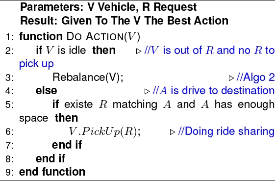
The internal state of the vehicle is composed of its position, represented by the latitude and longitude coordinates, its destination, and the number of seats empty. For an empty vehicle, the destination is zero, and if a vehicle responds to one or more requests, its destination corresponds to that of the request
A request R is available for a vehicle V if there are enough empty seats to accommodate the number of passengers associated with the request (ranging from 1 to 4), and the total waiting time for R, (i.e. the time between the creation of the request and the estimated time of passenger pick-up is less than the maximum time allowed; considered to be 15 minutes). All customers who have waited more than 15 minutes leave the system unserved, and the request is recorded as unserved.
Vehicles can choose between 3 actions, which are organized into two categories: (1) drop-off, in which a vehicle responds to a request by driving the passenger (s) to their destination, (2) pickup, in which a vehicle goes to a pickup point of the selected request, and (3) when the vehicle perception is empty, and it does not respond to any demand, it is activated to rebalance as shown in line 3 of the algorithm 1.
4.2 Rebalancer - DRBD
Rebalancing can be used for various carpooling systems; however, the researchers use the Expectation-Maximization approach for the clustering in their Deep RL carpooling request attribution strategy [5]. We only used DRBD rebalancing in our case, which is activated when a vehicle receives no requests and no more requests to serve in its region. The DRBD aims to allocate vehicles efficiently and dynamically based on current demand, thus avoiding fleet imbalance, leading to longer waiting times for passengers or a high number of requests not processed. DRBD deduces the travel zones and calculates their associated probabilities for a vehicle to rebalance Eq. 6:
where
The principle of the method BRBD is illustrated in Figure 4, representing the rebalancing module. The demand dispatcher has a dual role: it selects the demands for vehicles according to time and seat availability and filters the demand for rebalancing, depending on the period used.

Fig. 2 Observed demand imbalance in NY Taxi dataset [20] trips between morning (7-10 am) and evening (6-9 pm) in the south part of Manhattan on Tuesday, July 7, 2016 (evening)


DRBD takes as input the pending requests available at the moment. As shown in Figure 5, only the validated requests are considered, not any previous fulfilled or rejected requests (estimated or planned).
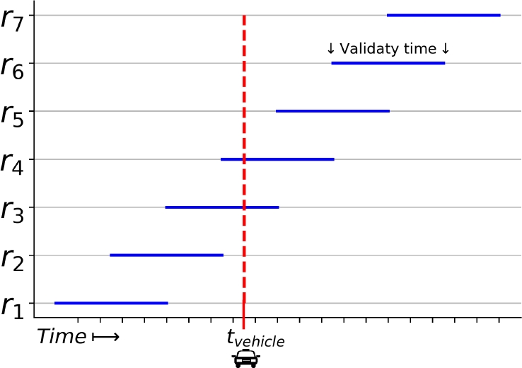
The procedure applied to move an idling vehicle to a new position is described in Algorithm 2. First of all, DRBD generates new clusters based on pending (unserved) requests, according to Algorithm 3.

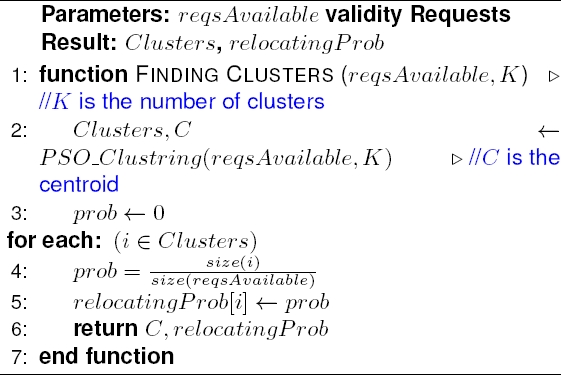
By applying optimization swarm particulates for clustering, a total of K clusters and their centroid are generated.
The vehicle is then moved to a featured area selected by a weighted random selection based on the probability of each category calculated in Equation 6 (lines 4-5. We preferred a weighted random selection approach over the others because it allows vehicles to explore different areas when rebalancing, preventing all vehicles from rebalancing in the same area.
5 Experimental Setup
The requests are generated using the Open New York Taxi Dataset [20]. It describes the recorded trips of yellow taxis in the Manhattan area. We extracted trips from three consecutive Tuesdays of July 2015 to represent typical weekday demand patterns.
We use a fixed fleet size of 200 shared vehicles to observe cases where the activation of carpooling is necessary to satisfy all requests (peak hours from 7:00 to 10:00). Each vehicle has a capacity of 4 passengers. Each request includes the time when the user requested the trip(ptime), the number of passengers(npass), the longitude and latitude of origin point (olng,olat), and the destination point (dlng, dlat) (See Table 1).
Table 1 Data set head
| N | ptime | olng | olat | dlng | dlat | npass |
| 1 | ||||||
| 1 | ||||||
| 2 |
We used a simplified traffic simulation to focus only on rebalancing and carpooling strategies without taking congestion into account. Vehicles drive themselves to their current destination (e.g., driver pick-up or drop-off point or relocation area).
Travel time is calculated in the same way as in a grid network, and we assume a speed of 35 Km/h for peak hours. The evaluation is based on morning peak traffic data (7:00 to 10:00) and includes 10,000 requests. The number of Passengers by request is distributed during evening peak time (See Figure 6).
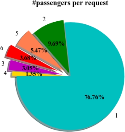
The demand satisfaction rate was less than 100%. Looking at Figure 6, it is apparent that few requests have 5 and 6 passengers necessitating the use of vehicles with 6 seats available together. All the vehicles used in the simulation had a maximum capacity of four passengers.
6 Results and Analysis
6.1 General Considerations
The DRBD rebalancing was compared with the following strategies to evaluate the performance of our approach:
— Base: a central dispatcher assigns the nearest vehicle to the request with the highest waiting time.
— Ride sharing: if the new request origin and destination are in zones on the current route, a vehicle can pick up more demands before it reaches full occupancy.
— Ride sharing and rebalancing: the vehicle drives towards the center of the zone to which it was randomly assigned.
For all the simulation scenarios, we have assumed that each vehicle has a capacity of 4 passengers, so requests with more than 4 passengers are ignored by the vehicles. Based on the data collection, the fleet will serve 90.85% of the 10,000 requests at its maximum level of service.
6.2 Evaluation Metrics
To evaluate DRBD, we use the set of the most commonly used indicators in related work:
— Number and percentage of served requests.
— Number and percentage of timed-out requests
— Waiting time
— Total Vehicle distance traveled per vehicle in service
— Number of requests served per vehicle
6.3 Simulation Results
Each scenario shows a different level of service according to the indicators mentioned above.
— Served requests: Scenario Base (no RB, no RS), which models a standard taxi service, serves about 83.88% of requests, and ride sharing serves 90.10% of requests. However, the DRBD serves 90.25% of requests.
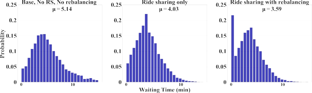
— Waiting time (WT): Passenger waiting times for each scenario were shown in Figure 7. We observed a significant reduction in waiting time by enabling ride sharing in the base scenario (No RS and No RB). RS only indicates waiting times (4.02 minutes); but, when we use PSO’s DBRB clustering, we see another reduction in WT (3.59 min).
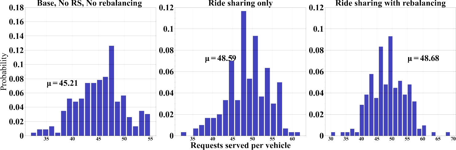
— Requests Distribution: As shown in Figure 8, several vehicles in the Base are traveling with just a few passengers in Base (no RB, no RS). Once serving one or few requests, these vehicles may end up in an area of the network that is empty of any further request. Enabling rebalancing or ride sharing can prevent them from staying idle and help the vehicle to find new requests. It can be seen in situations DRBD and ride sharing only, where allowing ride-sharing and rebalancing results in further improvements since all vehicles serve the same number of passengers.
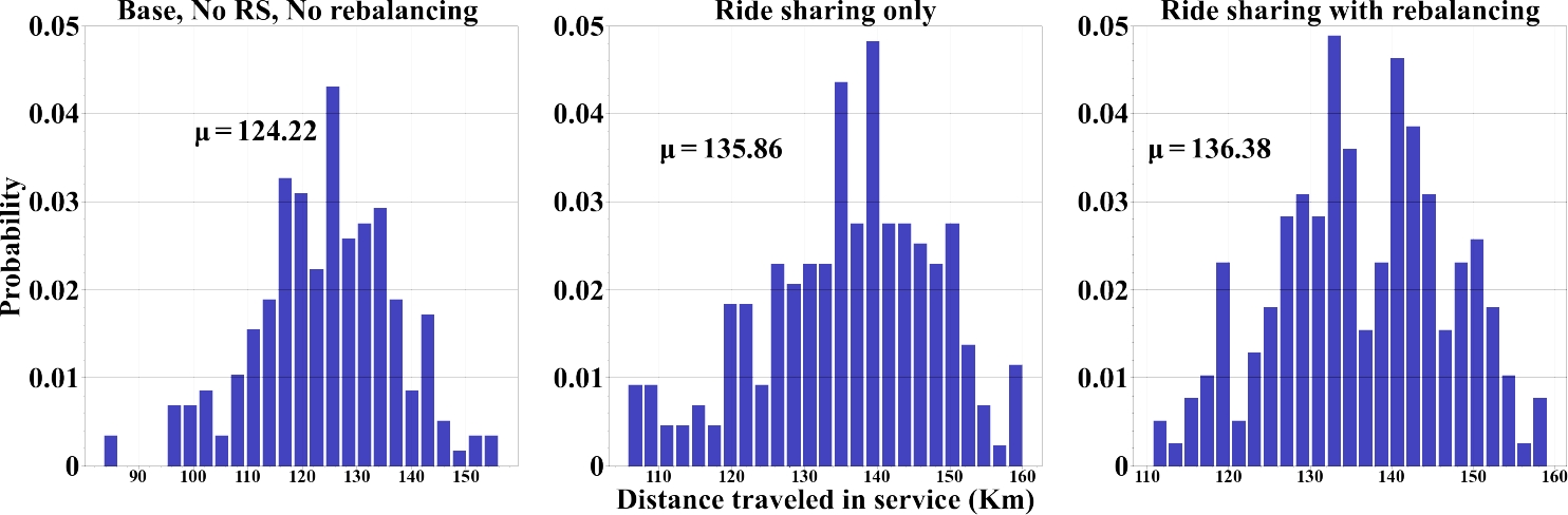
— Distance traveled: Figure 9 shows the distance traveled by vehicle for each scenario. Base scenario (no RB, no RS) shows that around one-fourth of the vehicles are traveling only a few kilometers, confirming they only serve a few requests and then stay idle in an area with no further demand. Since the number of serving requests varies by scenario, an essential difference in distance traveled was recorded. From Table 2, we can confirm that enabling rebalancing adds additional travel distance in service for vehicles.
6.4 Discussion
According to simulation results, allowing flight sharing and rebalancing has shown very positive results in satisfying most possible service requests. We showed that DRBD with PSO Clustering improves all vehicles’ average and individual performance when used in conjunction with ride sharing compared to Base (no RD, no RS).
Passenger wait time for DRBD has decreased to nearly 40% compared to classic taxi service (Scenario Base - no RB, no RS). However, the main observed advantage of DRBD (with RB and RS) is that each vehicle’s workload seems to better converge to a global average value, resulting in fairer workload distribution. It has been found that the rebalancing approach (RS and RB with DRBD scenarios) generates additional traveled distance, resulting in a slight increase in overall distance in operation.
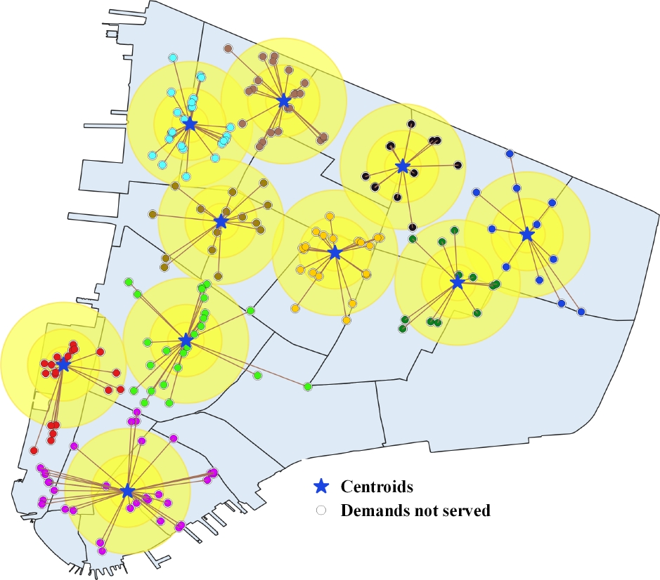
We show a snapshot of the number, size, and shape of the clusters it created for idle vehicle V at time t to illustrate how DRBD by PSO clustering differs from fixed zone clustering in terms of zone outcomes (See Figure 10). DRBD was used to calculate ten relocation zones in this case. The stars represent cluster centers, and the number of the related trips.
7 Conclusion and Future Work
This paper presents a Dynamic Rebalancing Based on Demand (DRBD), a vehicle rebalancing algorithm for ride sharing in sharing vehicle systems. Unlike existing approaches which use fixed geographical zone to relocate empty vehicles, DRBD uses PSO clustering to generate zones dynamically. DRBD enables zones to be dynamic in terms of position by their centroid.
First, rebalancing areas are identified by analyzing pending requests in real-time at each time step. The zone to which an unoccupied vehicle rebalances is then determined using a probability distribution defined on the zones, which is calculated by dividing the number of requests in the zone by the total number of requests in all zones.
The effectiveness of the BRBD is simulated by integrating it with 200 carpool vehicles, which respond to 10,000 carpool requests in the lower Manhattan area. In terms of the DRBD technique, the workload is distributed more evenly throughout the fleet, suggesting a more accurate rebalancing strategy with no loss of efficiency while respecting waiting times and passenger distribution by vehicle.
This work can be extended in several directions. Check for general applicability should be combined with other ride sharing methods and tested using other maps and data sets of road networks. In terms of learning, the vehicles could be activated using a reinforcement learning model to fine-tune their behaviors in response to new demand models that emerge. Rebalancing could be further improved by considering real-time traffic congestion when deciding which cluster to move.

