


 nueva página del texto (beta)
 Inglés (pdf)
 Artículo en XML
 Referencias del artículo
 Enviar artículo por email
 Citado por SciELO
  Similares en
SciELO
Similares en
SciELO 
 Permalink
1 Introduction
Recently, a new disease called COVID 19 (Coronavirus) appeared in December 2019 in Wuhan, the capital of Hubei, China. COVID 19 spreads near contaminated surfaces with an age ranging from several hours to several days depending on the nature of the surface, it spreads as well by coughing or sneezing (the virus can be transmitted to another person through saliva droplets).
This virus has several symptoms such as fever, cough, tiredness and in more advanced stages can lead to difficulty in breathing medically referred to as dyspnea.
On March 11th, 2020, the World Health Organization (WHO) declared a pandemic cannot be controlled. According to the Worldometer website, there have been 259,645,518 cases touched by the virus and 5,190,691 deaths.
In this case, if we want to prevent or at least reduce the spread of this disease, we must try something that can speed up the diagnosis.
So, the idea is to find out if an individual is infected with the coronavirus in the early stages that it is easier to deal with and the contagion can be stopped. Among the used solutions is the intercalation of Deep learning in the medical field.
Deep Learning precisely convolutional neural networks (CNN), has rapidly become the method of choice for the analysis of radiological images.
In general, the convolutional neural network process includes the feature extraction phase, yet it requires a huge amount of input images for the network to be capable of learning.
Providing data needs a lot of time but as is mentioned previously the more time we take, the more the epidemic spreads. Several works have been done in deep learning for medical diagnosis as discussed below.
In [1], the authors proposed a combination of deep learning, natural language processing, and medical imaging to improve medical diagnosis. This work is a survey of deep learning in medical diagnosis. In [2] the authors present a survey of the therapeutic areas and deep learning models for diagnosis. In [3] the authors present an overview of the deep learning approach for COVID 19 diagnosis. In [4], Medjahed et al proposed a new approach for COVID-19 diagnosis based on feature selection and meta-heuristic called Multi-Verses Optimizer.
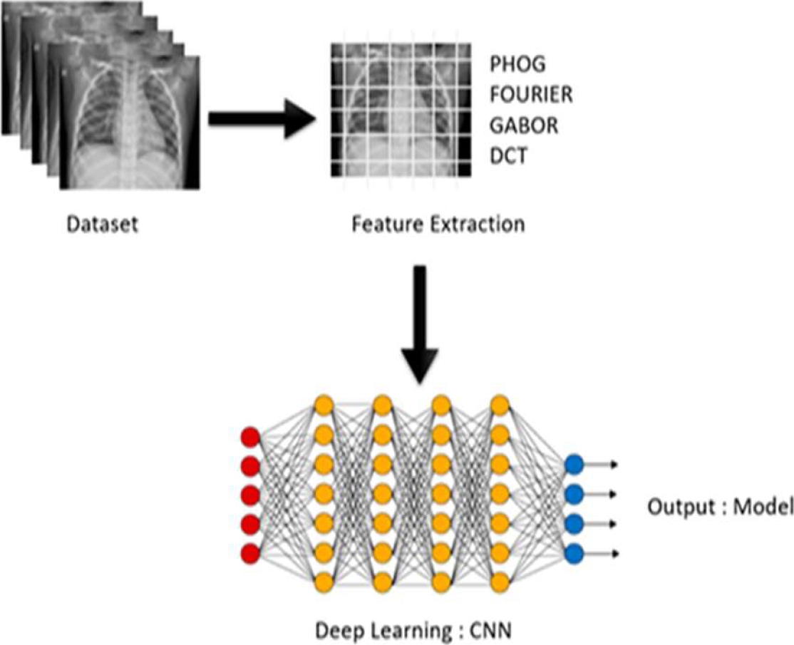
In our approach, the main idea consists of combining feature extraction and deep learning to enhance the quality of medical diagnosis and to give a better performance. We will introduce the two main keys of Deep Learning and feature extraction.
The first one is the representation of an image as a vector of features, among the methods of feature extraction, we cite Pyramid Histogram of Gradient, Local binary patterns, Color histograms, Fourier, Gabor, Discrete cosine transform, etc. In our work, we propose to use four of the most relevant feature extraction methods to extract the features of the image dataset: Pyramid Histogram of Gradient, Fourier, Gabor, and Discrete cosine transform. Secondly, we train CNN with the data gained from the first step by introducing the features extracted.
The experiment is conducted on x-ray images of people infected with the Corona epidemic and others who are not infected.
The rest of this paper is organized as follows. Section 2 presents the state of the art of feature extraction and deep learning. Section 3 illustrates the proposed approach. Section 4 presents the experimental results. Section 5 draws some perspective.
2 State of the Art
2.1 Feature Extraction
In this section, we have focused on four feature extraction methods used in our work:
Histogram of The Pyramid Orientation Gradients (PHOG), divides the image into sub-regions that have different resolutions, it is generally used for object detection [4, 7].
Histograms of oriented gradients are feature descriptors used for object detection. It was first introduced by Navneet Dalal and Bill Triggs, researchers for the French National Institute for Research in Computer Science and Control (INRIA), [10].
The technique works by counting the occurrence of gradient orientation computed on a dense grid of uniformly spaced cells on an image. The idea behind this algorithm is that the local appearance of objects in an image can be described using the distribution of edge directions. The HOG descriptor is, in particular, useful for pedestrian detection [11].
Pyramid histogram of gradients (PHOG) is an extension to HOG features. Extending HOG to PHOG is by analogy very similar to the extension of HOW (histogram of visual words) to PHOW. In PHOG, the spatial layout of the image is preserved by dividing the image into sub-regions at multiple resolutions and applying the HOG descriptor in each sub-region.
To program the PHOG features, the Canny edge detector is usually applied on grayscale images, then a spatial pyramid is created with four levels [12]. The histogram of oriented gradients is then calculated for all bins in each level. All histograms are then concatenated to create the PHOG representation of the input image.
Fourier Functions
Fourier function is widely used in image processing. It is divided into sine and cosine components. The number of pixels in the image represents the number of frequencies [4, 7].
Fourier transform is a mathematical function that decomposes a waveform, which is a function of time, into the frequencies that make it up.
The result produced by Fourier transform is a complex-valued function of frequency. The absolute value of the Fourier transform represents the frequency value present in the original function and its complex argument represents the phase offset of the basic sinusoidal in that frequency.
Fourier transform is also called a generalization of the Fourier series. This term can also be applied to both the frequency domain representation and the mathematical function used.
Fourier transform helps in extending the Fourier series to non-periodic functions, which allows viewing any function as a sum of simple sinusoids.
Gabor Feature
This method combines the characteristics of scale, spatial location, and orientation to recognize a region [4, 7].
This feature relies on using Gabor filters for character recognition in gray-scale images is proposed in this paper. Features are extracted directly from gray-scale character images by Gabor filters which are specially designed from statistical information of character structures.
An adaptive sigmoid function is applied to the outputs of Gabor filters to achieve better performance on low-quality images. To improve the discriminability of the extracted features, the positive and the negative real parts of the outputs from the Gabor filters are used separately to construct histogram features.
Experiments show us that the proposed method has excellent performance on both low-quality machine-printed character recognition and cursive handwritten character recognition.
Discrete Cosine Transforms (DCT)
DCT divides the image depending on the visual into sub-blocks of different importance [4, 7].
The discrete cosine transform (DCT) is a real transformation that has great advantages in energy compaction. Its definition for spectral components DP u,v is:
There are many variants of the definition of the DCT, and we are concerned only with principles here. The inverse DCT is defined by:
A fast version of the DCT is available, like Fourier Functions Transform (FFT), and calculation can be based on the FFT. Both implementations offer about the same speed. The Fourier transform is not optimal for image coding since the DCT can give a higher compression rate, for the same image quality. This is because the cosine basis functions can afford high-energy compaction.
2.2 Deep Learning
Deep learning is a sub-domain of machine learning, it concerns algorithms inspired by the structure and function of the human brain. These algorithms are called artificial neural networks (ANNs). Deep learning consists of neural networks with a large number of layers and parameters.
There are three fundamental network architectures: artificial neural networks (ANNs), recurrent neural networks (RNN), recursive neural networks, and convolutional neural networks (CNN). The automatic feature extraction is one of the main facets, indeed, summarizing this step to a simple raw image introduction seems like one of the great advantages of deep learning [8].
Activation Function
It matches the inputs of a node to its corresponding output, e.g., Sigmoid, Tanh, ReLU, etc. These functions are constructed using different mathematical techniques.
There are several types of activation functions, but the most popular activation function is the rectified linear unit function, also known as the ReLU function.
It is well-known to be a better activation function than the sigmoid function and the Tanh function because it performs the descent of the slope faster. Indeed, in the sigmoid and Tanh function when the input (x) is very large, the slope is very small, which slows down the descent of the gradient considerably [8].
Cost Function
Similar to any other machine learning model, it measures the "quality" of a neural network in relation to the values it predicts in relation to the actual values. The cost function is inversely proportional to the quality of a model - the better the model, the lower the cost function. In other words, the more the cost function is minimized, the more the weights obtained and the parameters are optimal for the model, resulting in a powerful model.
There are several commonly used cost functions, including quadratic cost, cross-entropy cost, exponential cost, Hellinger distance, Kullback-Leibler divergence [8].
Back Propagation (BP)
BP algorithm is a method to monitor learning. It utilizes the methods of mean square error and gradient descent to realize the modification to the connection weight of the network.
The modification to the connection weight of the network is aimed at achieving the minimum error sum of squares. In this algorithm, a little value is given to the connection value of the network first, and then, a training sample is selected to calculate the gradient of error relative to this sample [9].
2.3 Fundamentals Network Architectures
In this section, we have focused on the three basic network architectures known in deep learning and have briefly explained their principles:
Recurrent Neural Networks
A Recurrent Neural Network (RNN) is known for its ability to ingest inputs of varying sizes. They take into account both the current input and the previous inputs given to it, meaning that the same input can technically produce a different output based on the previous input data. In RNNs the connections between nodes form a digraph along a time sequence, allowing them to use their internal memory to process sequences of inputs of variable length.
RNNs are a type of neural network that is mainly used for sequential data or time series [8].
Long-term and Short-term Memory Networks (LSTM)
Created to fill one of the gaps in ordinary RNNs, they have a short-term memory. Specifically, if a sequence is too long, i.e., if there is a time lag of more than 5-10 steps, LSTMs tend to reject information that has been provided in previous steps. The LSTMs has therefore been created to solve this problem of Vanishing gradient [8].
Convolutional Neural Networks
A convolutional neural network (CNN) is a type of neural network that takes an input (usually an image), assigns importance to different features in the image, and produces a prediction.
What makes CNN's better than forward neural networks (FNN), they are better at capturing spatial dependencies (pixels) throughout the image, which means they can better understand the composition of an image.
CNN's uses a mathematical operation called convolution. In the literature, convolution is defined as a mathematical operation on two functions that produces a third function expressing how the shape of one is changed by the other.
This convolution is used by CNNs instead of the matrix multiplication in at least one of their layers. CNN's are mainly used for image classification [8].
3 Proposed Approach
Based on what we have mentioned in the previous section, we have decided to use CNN reason of its effective results on a dataset containing images specially on classification problems.
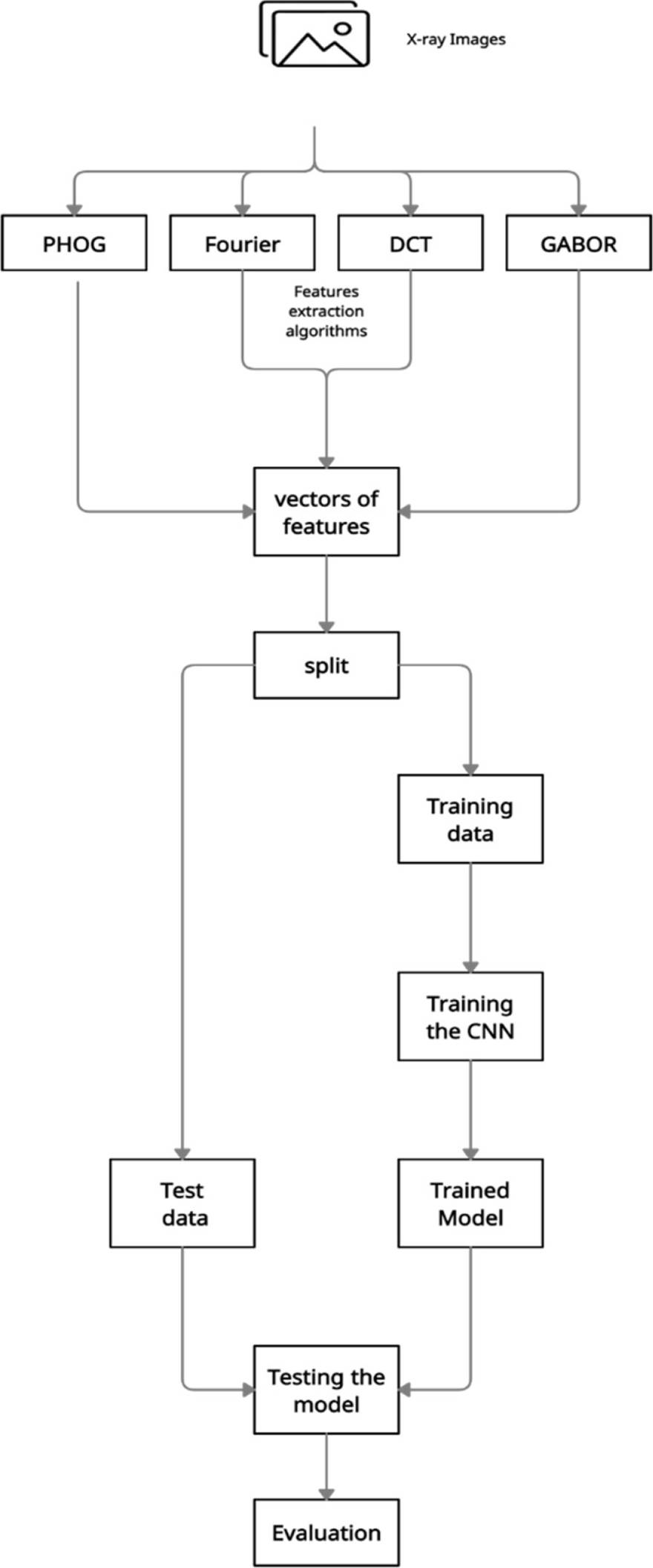
The approach is divided into four phases (Fig. 4):
− Data preprocessing phase,
− Model training phase,
− Model testing phase,
− Model evaluation phase.
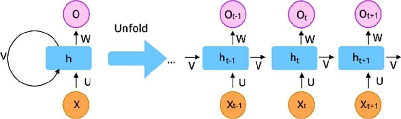
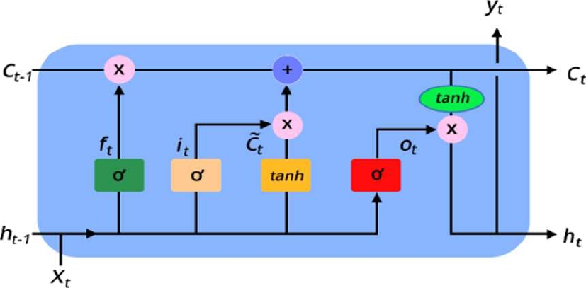
Fig. 2 Long short-term memory neural network, Image provided via improving long-horizon forecasts with expectation-biased LSTM networks

3.1 Data Preprocessing Phase
First of all, the data we are going to utilize must be well prepared for the training phase, to be so, many functions will be applied to this data, and these functions are the following:
− Reading the grayscale images from two folders, each folder contains 25 images (images are in black-and-white color).
− Adding the label of each image in a [-1] Data-frame, the value is 1 if the person has Coronavirus and 0 if he is not having the virus (Target Data-frame).
− Applying image features extraction algorithms on each uploaded image (PHOG, DCT, FOURIER, GABOR). Each algorithm of the four mentioned algorithms takes an image as input and its output is a vector.
− Concatenating all the produced vectors to one single data frame, each row of this Data-frame is a vector.
− At this level, we obtain two Data-frame, the target Data-frame, and the new converted Data-frame.
− Concatenating these two Data-frame to one dataset.
− Choosing randomly 70% of data for the training process assuring that this 70% has 50% of each label target and the left 30% for the test phase.
− Finally, splitting the training dataset into X_train and Y_train and the test dataset into X_test and Y_test.
3.2 Model Training Phase
This phase consists of using the CNN model for the training model with the 70% dataset from phase A. the model architect is defined to many layers as below:
− The first layer is the input layer used to read and normalize the data.
− The second layer multiplies input data by weight and adds a bias vector.
− The Batch normalization layer is applied to allow every layer of the network to do learning more independently.
− The fourth layer uses the rectified linear unit.
− The Fifth layer multiplies the data by weight and adds a bias vector, in this layer using the SoftMax activation function.
− The last layer is the classification layer that produces given outputs (0 or 1).
The phases A and B are illustrated in Fig. 5.
3.3 Model Testing Phase
This phase consists of testing the trained model from phase B utilizing a 30% dataset from phase A.
3.4 Model Evaluation Phase
This phase is about evaluating the model using classification metrics such as Confusion Matrix, Accuracy, Precision, Sensitivity, and Specificity.
These metrics help us to be able to compare the results of different classification models (Our approach, SVM, KNN, NB).
We will show in section 4 that our approach gives the best results.
4 Experimental Results
In this section, we present the experimental results obtained by the proposed approach and compare them to several classification methods.
4.1 Dataset Collection
The used dataset in this experience is collected by Adrian Rosebrock and it is available on Pyimageseach websitefn.
The data is composed of 50 images of chest X-rays and it is divided into two categories: 25 images of healthy people and the rest are those who have Covid19 [5], [6].
The images used in this work are illustrated in Fig. 6.
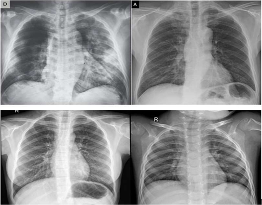
The figure shows the images used for experimentation. The first row is a normal image and the second row shows a Covid 19 image.
4.2 Dataset Collection
Generally, in deep learning, it is common knowledge that too little training dataset results in a poor approximation, underfit the model, and poor performance but our approach demonstrated that it can train a model with a small dataset.
The proposed approach is compared with other machine learning classification algorithms using accuracy metrics.
Support Vector Machine (SVM), K-Nearest Neighbor (KNN), and Naïve Bayes (NB) are used with the same training, test datasets that we used in our approach.
Table 1 illustrates the results of this study compared to other methods.
Table 1 The results of this study compared to other methods
| Proposed method (FE-DL) | Support Vector Machine (SVM) | K-nearest neighbor (KNN) | Naïve Bayes (NB) | |
| Worst (%) | 92.24 | 80.88 | 65.21 | 83.60 |
| Best (%) | 92.95 | 81.68 | 66.25 | 84.26 |
| Average (%) | 92.43 | 81.43 | 65.58 | 84.12 |
| Standard Deviation |
± 0.074 |
± 0.14 |
± 0.13 |
± 0.11 |
Classification accuracy is reported in Table 1. The second column presents the results obtained by the proposed approach.
FE-DL, the third column represents the results obtained by SVM, the fourth column is the results obtained by KNN and the last column presents the results obtained by Naïve Bayes.
We have run 100 times, each time containing 100 iterations for all the models (FE-DL, SVM, KNN, NB) and we have recorded the worst, the average, and the best accuracy values. We have also calculated the standard deviation in order to be able to see if the model's training is stable or not.
As we have seen in Table 1, the proposed approach produced a high classification accuracy rate competed to other approaches. We note 92.43% of the average classification accuracy rate. The best value is 92.95% and the worst value is 92.24%.
Naïve Bayes (NB) has provided a good result, the average is 84.12%, the worst is 83.60% and the best is 84.26%. We record for SVM 81.68% for the best classification accuracy rate, 80.88%, for the worst, and 81.43% for the average value. KNN has produced no satisfactory results, the average is 65.62%, the worst is 65.21% and the best is 66.25%.
The best value of standard deviation is noted for FE-DL and SVM approaches. Fig. 7 describes the results obtained by all the approaches versus the number of executions.
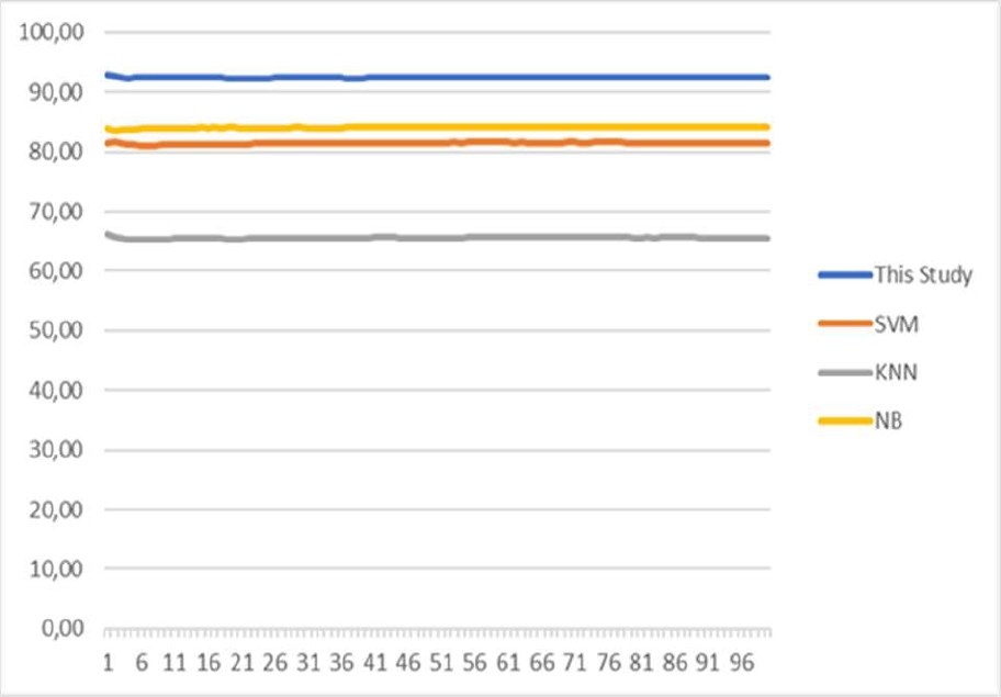
We clearly remark that the proposed approach is very stable, even if the training and testing set changed.
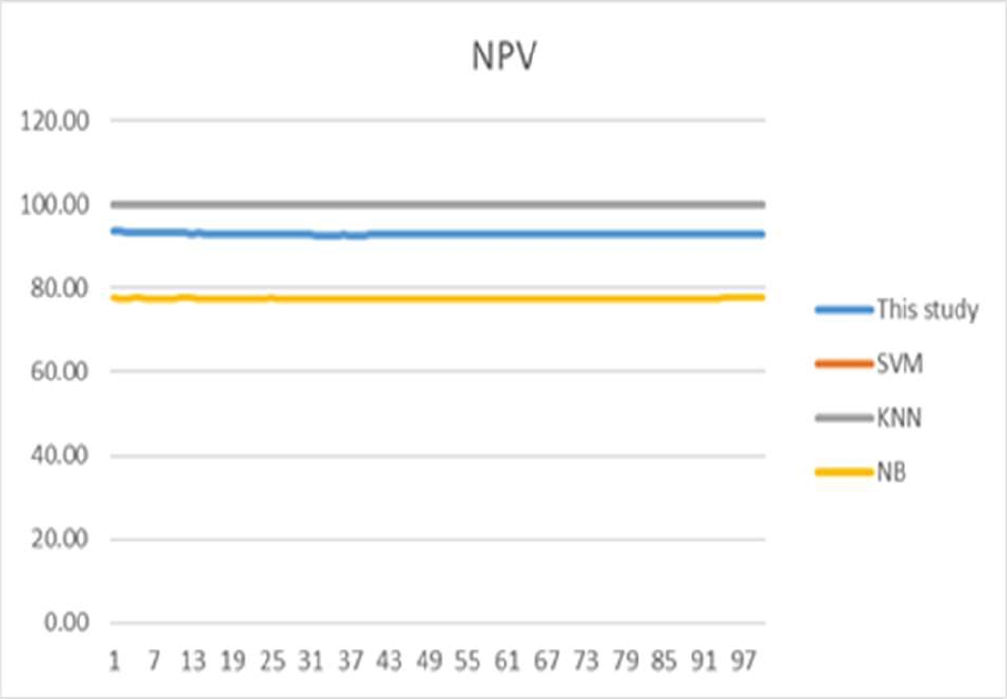
In order to outperform the stability and the performance of the proposed approach, we calculated the negative predictive value (NPV) and the positive predictive value (PPV), also the sensitivity and specificity. Fig. 8, 9, 10, and 11 illustrate the last values.


Sensitivity called also "Selectivity" and Specificity are two important parameters used for medical diagnosis. Sensitivity measures the ability to give positive results when the instance is verified. Specificity is opposed to sensitivity; it measures the ability to give negative results when the instance is not verified.
Sensitivity and Specificity can be seen as probability and a rate of a dataset.
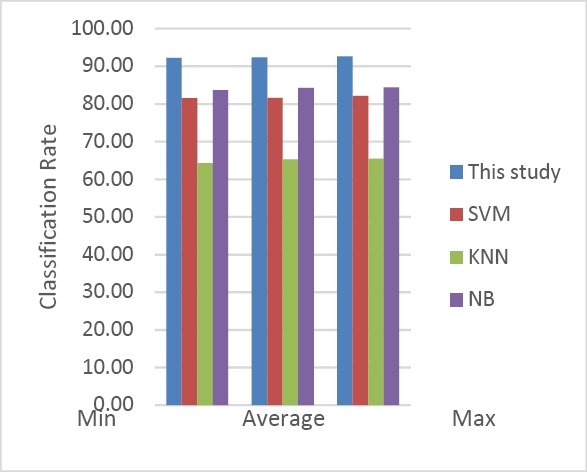
The analysis of the obtained results shows that the proposed approach is efficient. We remark a 92.15% minimum classification rate and 95.55% as maximum classification rate over the 100 run times.
In this case, we can say that the proposed approach is more stable. For SVM we note an 81.47% for the minimum and 82.12% as a maximum. The worst results are obtained by KNN with a 64.20% minimum of classification rate and 64.41% as maximum.
Fig. 8, 9, 10, and 11 show the PPN, NPV, Sensitivity, and Specificity obtained by the proposed approach and compared to SVM, KNN, and NB for all execution times. The proposed approach has provided a satisfactory result compared to the other approaches. We note that Sensitivity is the percentage of true positive and Specificity is the percentage of the true negative. PPV and NPV are used to determine the likelihood of a diagnostic test.
To analyze the performance of the proposed architecture in-depth, we propose to compare each feature extraction approach without combination.
We run the algorithm 100 times using PHOG, Fourier, GABOR, and DCT, and we record the minimum, average, and maximum classification accuracy rates. In addition, the proposed approach is compared to VGG16, which is a convolution neural network (CNN) considered as the best model architecture for deep learning. VGG16 was proposed by K. Simonyan and A. Zisserman [15].
Table 4 and Figure 13 illustrate the obtained results. Table 4 and figure 13 show the worst, best, and average classification accuracy rate obtained by the proposed approach and compared to each feature extraction approach and VGG16.
Table 2 Definition of the positive test and negative test
| Sick patients | Not-sick patient | |
| Positive test | True Positive | False Positive |
| Negative test | False Negative | True Negative |
Table 3 Maximum, average, and minimum values of specificity
| Proposed method (FE-DL) | Support Vector Machine (SVM) | K-nearest neighbor (KNN) | Naïve Bayes (NB) | |
| Worst(%) | 92.15 | 81.47 | 64.20 | 83.68 |
| Best(%) | 92.33 | 81.58 | 65.27 | 84.19 |
| Average (%) | 92.55 | 82.12 | 65.41 | 84.36 |
Table 4 Maximum, average, and minimum values of classification accuracy rate
| Classification Accuracy rate (%) | |||
| Worst | Best | Average | |
| Proposed Approach | 92.24 | 92.95 | 92.43 |
| Proposed Approach with PHOG | 91.10 | 92.05 | 91.42 |
| Proposed Approach with Fourier | 81.65 | 83.17 | 81.83 |
| Proposed Approach with GABOR | 89.62 | 89.96 | 89.77 |
| Proposed Approach with DCT | 77.02 | 77.99 | 97.22 |
| VGG16 | 93.01 | 93.52 | 93.29 |
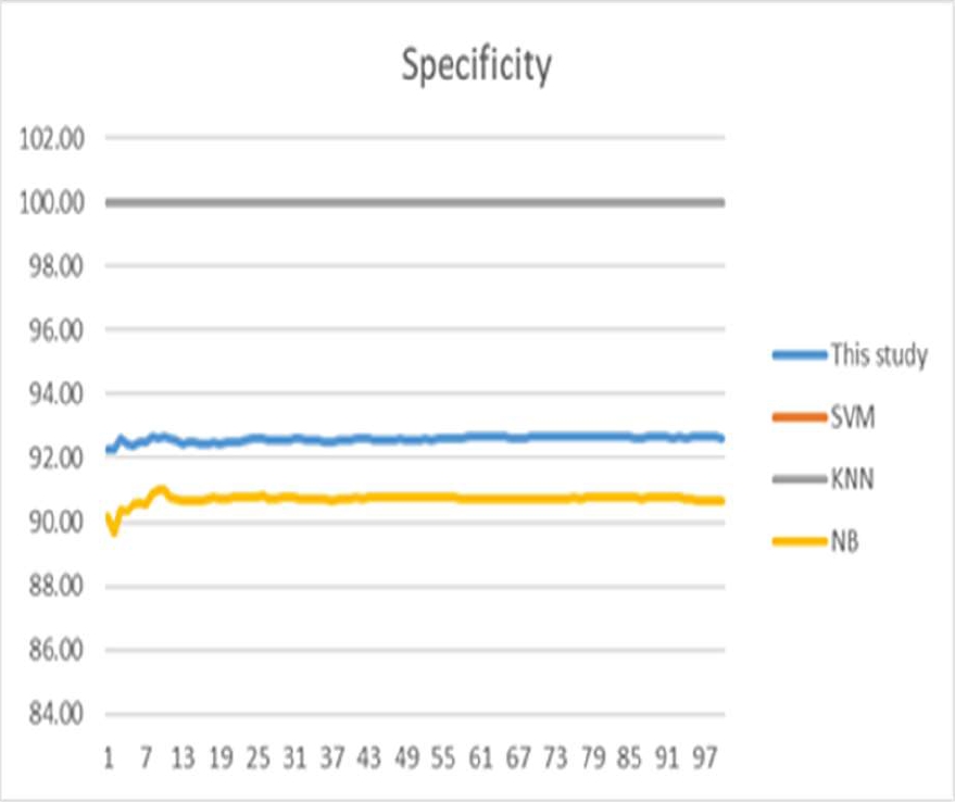
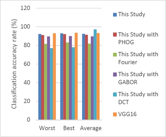
Fig. 13 Classification accuracy rate obtained by the proposed approach compared to each feature extraction method and VGG16
The analysis of results shows that the proposed approach provides satisfactory results compared to others.
The best result is recorded for VGG16 with 93.52% of classification accuracy and compared to the proposed approach, which provides 92.95% of classification accuracy rate. VGG16 is slightly higher than the proposed approach.
The worst results are obtained using DCT. In addition, PHOG produces a high classification accuracy rate compared to Fourier, Gabor, and DCT.
As future work, we can combine VGG16 with the proposed approach to improve the image classification accuracy.
5 Conclusion
These last years, deep learning has been a very interesting method and active research in many fields. In this paper, we proposed a hybrid approach based on two phases. The first one is the extraction of features using PHOG, Fourier, Gabor, and DCT. The second phase consists of using deep learning to classify the images. The proposed approach is trained and tested on the X-ray images of Covid 19.
The experimental results demonstrate the performance of the proposed approach. The proposed approach was compared to SVM, KNN, and NB. The results show that the proposed approach FE-DL outperforms compared to the others.
Our approach could be so beneficial for further future that it can be used to solve real-life problems even though insufficient data especially in urgent cases where there is not enough time to collect the data for instance Covid 19 virus.

