Ensemble Recurrent Neural Network Design Using a Genetic Algorithm Applied in Times Series Prediction

Pulido, Martha; Melin, Patricia; Pulido, Martha; Melin, Patricia

doi:10.13053/cys-26-2-4251

Servicios Personalizados

Revista

Articulo

Indicadores

Citado por SciELO
Accesos

Links relacionados

Similares en SciELO

Otros
Otros

Permalink

Computación y Sistemas

versión On-line ISSN 2007-9737versión impresa ISSN 1405-5546

Comp. y Sist. vol.26 no.2 Ciudad de México abr./jun. 2022 Epub 10-Mar-2023

https://doi.org/10.13053/cys-26-2-4251

Articles of the thematic issue

Ensemble Recurrent Neural Network Design Using a Genetic Algorithm Applied in Times Series Prediction

Martha Pulido¹

Patricia Melin¹^*

¹1 Tijuana Institute of Technology, Mexico. martha.pulido@tectijuana.mx.

Abstract:

This paper shows a new method based on ensemble recurrent neural networks for time series prediction. The proposed method seeks to find the structure of ensemble recurrent neural network and its optimization with Genetic Algorithms applied to the prediction of time series. For this method, two systems are proposed to integrate responses ensemble recurrent neural network that are type-1 and Interval type-2 Fuzzy Systems. The optimization consists of the modules, hidden layer, neurons of the ensemble neural network. The fuzzy system used is of Mamdani type, which has five input variables and one output variable, and the number of inputs of the fuzzy system is according to the outputs of Ensemble Recurrent Neural network. Test are performed with Mackey Glass benchmark, Mexican Stock Exchange, Dow Jones and Exchange Rate of US Dollar/Mexican Pesos. In this way was shown that the method is effective for time series Prediction.

Keywords: Time series prediction; genetic algorithm; ensemble recurrent neural network

1 Introduction

Recurrent neural networks (RNNs) were already conceived in the 1980s. But these types of neural networks have been very difficult to train due to their computing requirements and until the arrival of the advances of recent years, their use by the industry has become more accessible and popular [², ³, ⁴, ⁵, ¹⁰].

A recurrent neural network (RNN) is one that can be connected to any other and its recurring connection is variable. Partially recurring networks are those that your recurring connection fixed [¹, ², ⁹, ¹¹, ¹⁴, ¹⁷].

Recurrent Neural Networks are dynamic systems mapping input sequences into output sequences [¹⁹, ²¹, ²², ²³].

The calculation of an input, in a step, depends on the previous step and in some cases the future step [³⁴, ³⁵, ⁴⁰, ⁴⁴]. RNN are capable of performing a wide variety of computational tasks including sequence processing, one-path continuation, nonlinear prediction, and dynamical systems modeling [³⁸, ⁴⁷, ⁴⁹, ⁵⁰, ⁵²].

The purpose of carrying out a time series analysis of this type is to extract the regularities that are observed in the past behavior of a variable that is, obtain the mechanism that generates it, and know its behavior based on it over time.

This is under the assumption that the structural conditions that make up the phenomenon under study remain constant, to predict future behavior by reducing uncertainty in decision-making [⁶, ⁷, ⁸, ¹², ²⁹].

The essence of this work, is propose a new algorithm to design time prediction systems, where recurrent neural networks are applied to analyze the data, also type-1 and interval type-2 fuzzy inference systems to improve the prediction of time series.

For this, we apply a search algorithm to obtain the best architecture of the recurrent neural network, and in this way test the efficiency of the proposed hybrid method [⁶, ⁷, ⁸, ¹², ²⁹].

Genetic algorithms have been applied to various areas, such as forecasting classification, image segmentation routes for robots stand out, etc.

Their hybridation with other techniques improves the results of energy price predictions, raw materials and agricultural products, that is why we apply them to this approach, since they are tools that help use predict a time series and find good solutions, we have previously done work with this metaheuristic and they have given us good results, for this reason we apply it to network optimization neural ensemble for time series.

This work describes the creation of the ensemble recurrent neural network (ERNN), this model is applied to the prediction of the time series [²⁸, ³¹, ³⁶, ³⁹, ⁴¹], the architecture is optimized with genetic algorithms, (GA) [¹⁶, ²⁶, ²⁷, ⁴⁶].

The results of the integration of the Recurrent Neural Network are integrated with type-1 and interval type-2 fuzzy systems (IT2FS), [³⁰, ³², ³³, ⁴³, ⁴⁸]. The essence of this paper is the proposed architecture of the ERNN and the optimization is done using Genetic Algorithms, (GA), applied to the prediction of time series.

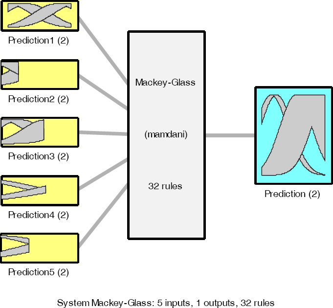
Two systems are proposed fuzzy type-1 and T2FS, to integrate the responses of the (ERNN), the optimization consists in the number of hidden layer (NL), their number of neurons (NN) and the number of modules (NM),) in the ERNN, the we integrate responses ERNN, with type-1 and IT2FS and in this way we achieve prediction. Mamdani fuzzy inference system (FIS) has five inputs which are Pred1, Pred2, Pred3, Pred4, and Pred5 and one output is called prediction.

The number of inputs of the fuzzy system (FS) is according to the outputs of ERNN. Mamdani fuzzy inference system (FIS) is created, this FIS five inputs which are Pred1, Pred2, Pred3, Pred4, and Pred5, (with a range) the range 0 to 1.4, the outputs is called prediction, the range goes from 0 to 1.4 and is granulated into two MFs "Low", "High", as linguistic variables.

This document is constituted by: Section 2 shows the database, in Section 3 the problem to be solved of the proposed model, Section 4 shows results of the proposed model, and Section 5 Conclusions.

2 Related Word

As related work, we can find a comparison was made using recurrent networks for the Puget Electric Demand time series, a learning algorithm was implemented for recurrent neural networks and tests were performed with outliers of data and in this way compare the capacity of loses, as well as the advantages of feedforward neural networks for time series are shown [¹⁸].

In [⁴⁵] a recurrent neural network was developed for prognostic problems; the time series of long memory patterns was used and tests were also carried out with the integrated fractional recurrent neural network (FIRNN) algorithm.

In another study it was shown the performance of the cooperative neuro-evolutionary methods, in this case Mackey-Glass, Lorenz and Sunspot time series, and also two training methods Elman recurrent neural networks [³⁷].

In another study, the prediction of time series was carried out, and the recurrent neural networks were used to make predictions. In this way the effectiveness of recurrent networks for the forecasting of chaotic time series was demonstrated [⁵¹].

In the study presented in [²⁰], Recurrent Neural Networks (RNNs), are used to model the seasonality of a series in dataset possess homogeneous seasonal patterns.

Comparisons with the autoregressive integrated (ARIMA) and against exponential smoothing (ETS), demonstrate that RNN models are not best solutions, but they are competitive.

In [⁵⁷], advanced neural networks were used for short term prediction.

Also, the exponential smoothed (ES) model for the time series are used, and this allows the equations to capture seasonality and the level more effectively, these networks allow trends non-linear and cross-learning, data is exploited hierarchically and local and global components are used to extract and combine data from or from a data series in order to obtain a good prediction.

This section shows the data set that was used to build the proposed model, in this case the Mackey-Glass time series are used.

2.1 Dataset Proposed

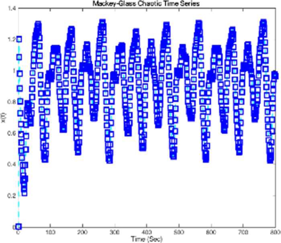
In this case we work the Mackey Glass time series with eight hundred data, we used 70% and 30% data for the training and testing, respectively. The following equation represents the Mackey-Glass time series:

x=0.2X(t−τ)1+X10(t−τ), (1)

where:

x(t)=0,

x(0)=1.2,

T=17,

t<0.

The plot of the Mackey Glass for the values mentioned in the equation is presented in Fig. 1. [²⁵, ²⁶].

Fig. 1 Plot of the Mackey-Glass Data Set

In Fig. 2, the graph of the Mexican Stock Exchange data [⁴²] is presented. In this case, we use 800 data that correspond to period from 01/04/2016 to 31/12/2019. We used 70% of the data for the RNN trainings and 30% to test the RNN.

Fig. 2 Plot of the Mexican Stock Exchange Dataset

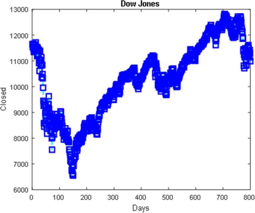
Fig. 3 presents the graph of the Dow Jones data [¹⁶], where we are using 800 data that correspond to period from 07/01/2017 to 09/05/2019. We used 70% of the data for the RNN trainings and 30% to test the RNN.

Fig. 3 Plot of the Dow Jones Dataset

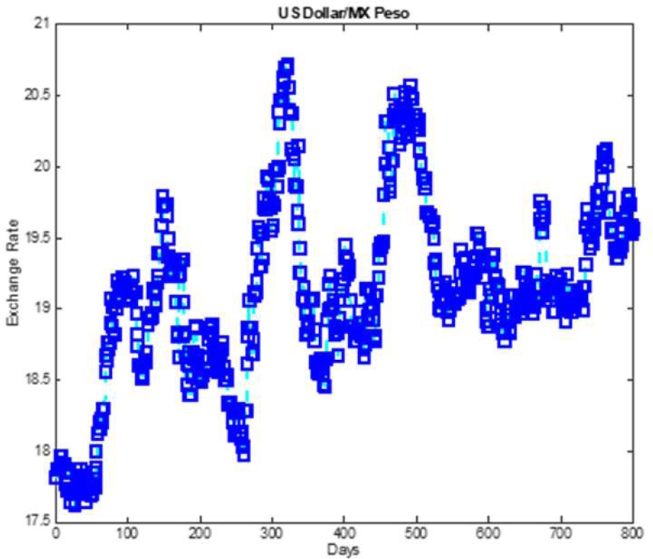
In Fig. 4 the graph of the data US Dollar/MX Peso [¹³] is illustrated, where we use 800 data that correspond to the period from 07/01/2016 to 09/05/2019. We used 70% of the RNN training and 30% to test the RNN.

Fig. 4 Plot of the US Dollar/MX Pesos

We trained the ensemble recurrent neural network with 500 data points, and we use the Bayesian regularization backpropagation method (trainbr) with a set of 300 points for testing, this is for each of the previously mentioned times series.

3 Problem Statement and the Proposed Method

In this Section, it is explained how the ERNN optimization model was created, its integration with type-1 and IT2FS, and we also describe every detail of the technique used for the optimization of the ERNN, as well as type-1 and IT2FS for the prediction of the time series.

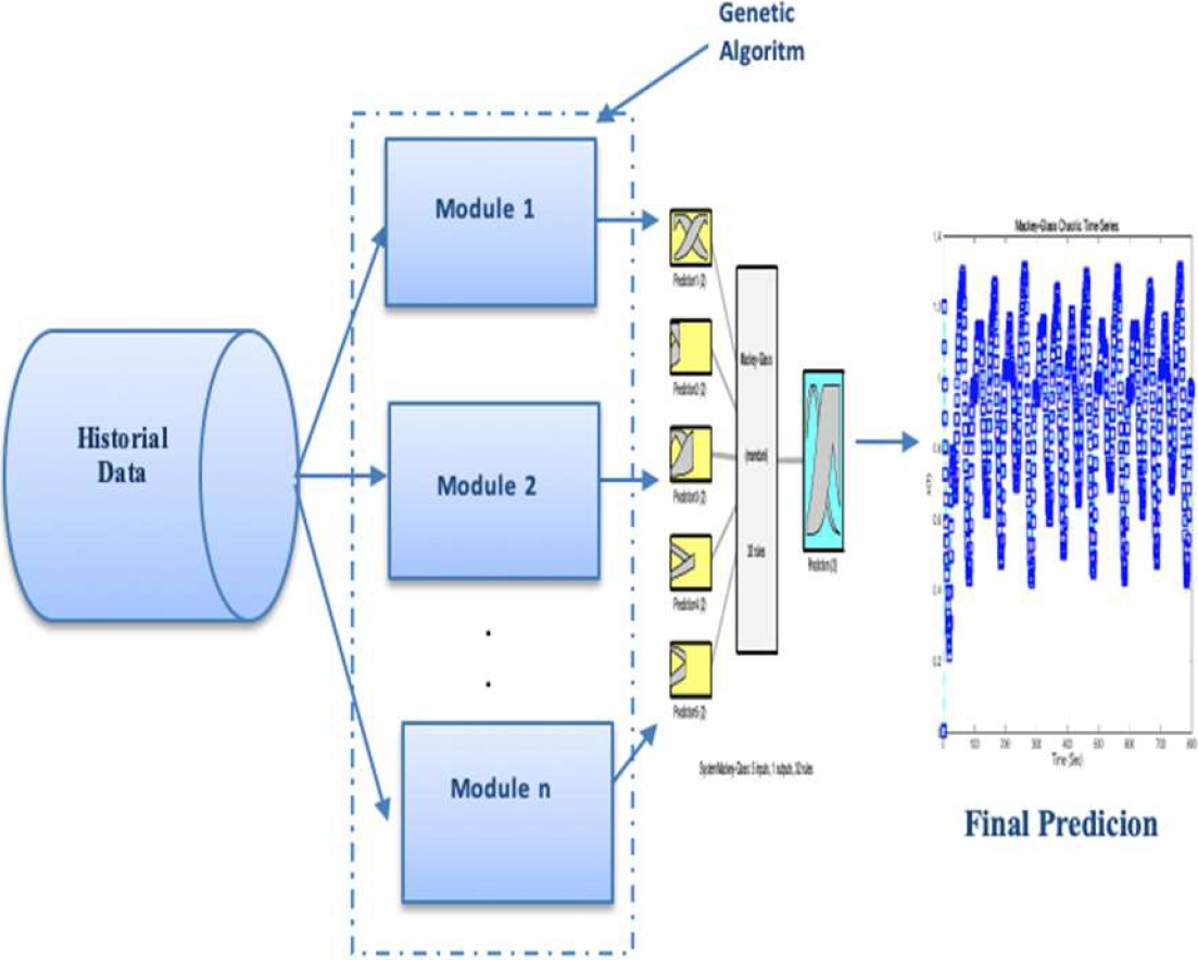
3.1 Proposed General Scheme

The first part is to obtain the dataset of the time series, the second part it is determining the number of modules ERNN with the genetic algorithm, and the third part would be to integrate with type-1 and T2FS type-2 the responses of the ERNN to finally achieve time series prediction, as can be observed in Fig. 5.

Fig. 5 Proposed General Scheme

3.1.1 Creation of the Recurrent Neural Network (RNN)

Recurrent neural networks (RNNs) have all the characteristics and the same operation of simple neural networks, with the addition of inputs that reflect the state of the previous iteration. They are a type of network whose connections form a closed circle with a loop, where the signal is forwarded back to the network, that is, the neural network’s own outputs become inputs for later instants. This feature endows them with memory and makes them suitable for time series modeling. The layer that contains the delay units is also called the context layer, as shown (as can be illustrated) in Fig. 6:

Fig 6 Recurrent Neural Network

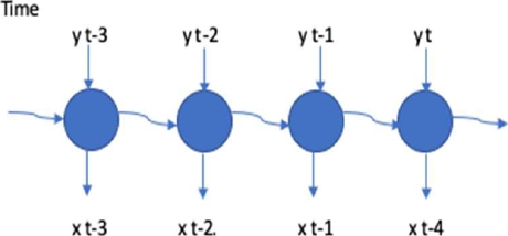
The recurrent neural network is made up of several units of a fixed activation function, one for each time step, each unit has a state and it is called the hidden state of the unit and it means that the network has past knowledge and a certain time step. This hidden state is updated and signifies the change in the network's knowledge about the past:

yt=fW(xt,ht−1). (2)

where ht−1 the old hidden state, ht represents the new hidden state, fW the fixed function with trainable weights and xt is the concurrent input.

The new hidden state is calculated at each time step, and recurrence is used as above and the new hidden state is used to generate a new state, and so on.

Where the input stream from the previous layer, the weights of the matrix, and bias already seen in the previous layers. RNNs extend this function with a recurring connection in time, where the weight matrix operates on the state of the neural network at the previous time instant. Now, in the training phase through Backpropagation, the weights of this matrix are also updated.

3.1.2 Description of the GA for RNN Optimizations

The parameters of the recurrent neural network that are optimized with the GA are:

Number of modules (NM).
Number of hidden layers (NL).
Number of neurons of each hidden layer (NN).

The following equation represents the objective function that (that is implemented in GA) we used with a genetic algorithm to minimize to prediction error of the time series:

ERM=(∑i=1d|pi−xi|)/dPrediction Error=(ERM1+ERM2+⋯+ERMN)/N. (3)

where p represents the predicted the data for each module of ensemble recurrent network, X corresponds to the real data of time series, 𝑑 is the number of data used by time series, ERM is the prediction error by module of ERNN, to 𝑁 corresponds the number of modules determined by the GA and the Prediction Error corresponds to average prediction error achieved by the ERNN.

Fig. 7 presents the structure of the GA chromosome.

Fig. 7 Chromosome Structure to optimize the RNN

The main goal to optimize the ERNN architecture, with a GA is to obtain the best prediction error, which seeks to optimize NM, NL, and NN of the ERNN. Table 1 shows the values of the search space of the GA.

Table 1 Table of values for search space

Parameters of RNN	Minimum	Maximum
Modules	1	5
Hidden Layers	1	3
Neurons for each hidden Layer	1	30

In Table 2, the values of the parameters used for each optimization algorithm are presented. The mutation value is variable and shown in Table 2.

Table 2 Table of GA parameters

Parameter	Value
Generations	100
Individuals	100
Crossover	Single Point
Probability	0.85
Selection	Roulette
Mutation	Variable

3.1.3. Description of the type-1 and IT2FS

The next step is the description of the type-1 fuzzy system and IT2FS. The following equation shows how the total results of the FS are calculated:

y=∑i=1nxiu(xi)∑i=1nu(xi)i, (4)

where u represents the MFs and x corresponds to the input data.

Fig. 8 shows a Mamdani fuzzy inference system (FIS) that is created. This FIS has five inputs, which are Pred1, Pred2, Pred3, Pred4, and Pred5, the range 0 to 1.4, the output is called prediction and the range goes from 0 to 1.4 and is granulated into two MFs "Low", "High", as linguistic values.

Fig. 8 IT2FS

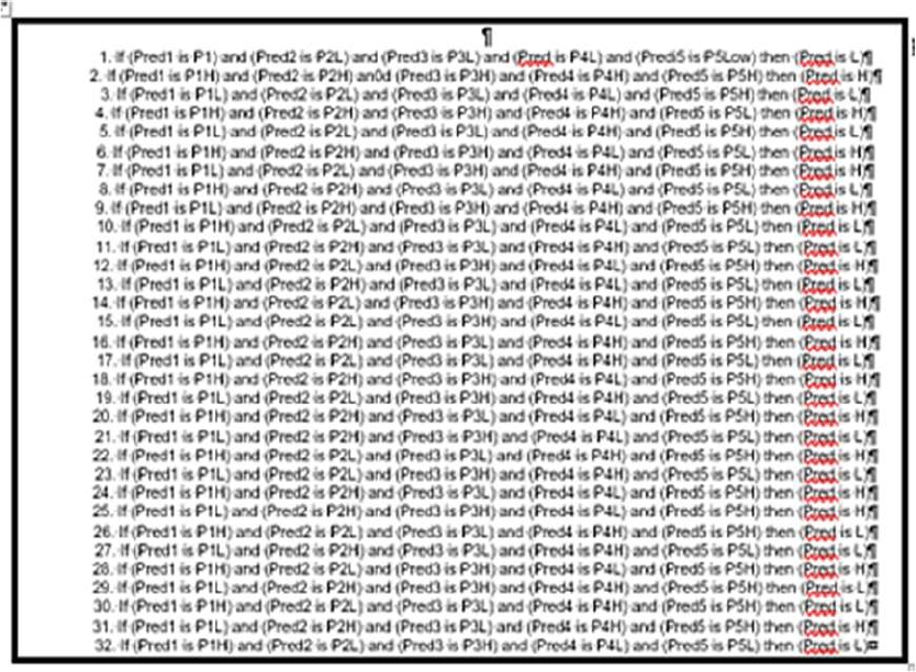
The Fuzzy system rules are as follows (as shown in Figure 9), since the fuzzy system has 5 input variables with two MFs and one output with two MFs, therefore the possible number of rules is 32.

Fig. 9 Rules used for the IT2FS

4 Experimentation Results

This part presents the experiments of the optimization of the ERNN with the GA, as well the integration type-1 and IT2FS.

In addition, we present graphs of real data against predicted and results of the prediction for each of the experiments of Mackey Glass benchmark, Mexican Stock Exchange, Dow Jones, and Exchange Rate of US Dollar/Mexican Pesos time series. The following table shows the results of the genetic algorithm, where the best architecture of the ERNN is shown in row number 7 of Table 3 for the Mackey-Glass time series.

Table 3 Genetic algorithm results for the RNN of MG

Evolutions	Gen.	Ind.	Pm	Pc	Num. Modules	Num. Layers	Num. Neurons	Duration	Prediction Error
1	100	100	0.07	0.6	3	2	22,23 18,19 17,16	05:10:11	0.0017568
2	100	100	0.05	0.7	5	2	18,22 23,24 25,26 20,21 18,20	06:22:16	0.0019567
3	100	100	0.07	0.5	4	2	25,26 20,22 24,25 21,22	07:24:22	0.0020174
4	100	100	0.03	0.4	5	2	18,22 23,24 25,26 20,21 18,20	07:36:27	0.0016789
5	100	100	0.09	0.9	3	2	18,22 21,22 15,16	06:15:16	0.0017890
6	100	100	0.05	0.5	5	2	19,20 23,24 25,26	09:35:23	0.0020191
7	100	100	0.09	0.9	3	2	24,25 23,22 20,21	0:06:17	0.0015678
8	100	100	0.09	1	5	2	19,18 21,22 27,28 24,24 21,22	06:12:11	0.0018904
9	100	100	0.04	0.7	4	2	19,20 21,22 25,25 18,22	06:13:34	0.0855
10	100	100	0.03	0.7	5	3	20,19,22 18,19,19 22,24,27 21,19,20 26,25,26	08:20:19	0.0016311

Table 4 illustrates the results of the type-1 FS integration for the optimized ERNN, where the obtained result is of experiment number 8, with a prediction error: 0.1667. Figure 9 represents the plot of the real data against predicted data for the type-1 fuzzy system for the Mackey-Glass time series. Table 5 and Figure 10 represent the prediction of the time series using the IT2FS for the Mackey-Glass time series, respectively. Table 6 shows the results of the genetic algorithm, where the best architecture of the ERNN is shown in row number 2 of Table 6 for the Mexican Stock Exchange time series.

Table 4 Results of type-1 FS for MG

Test	Prediction Error with Type-1 Fuzzy Integration
1	0.1731
2	0.2012
3	0.1965
4	0.2034
5	0.1886
6	0.2898
7	0.2234
8	0.1667
9	0.1945
10	0.2225

Fig. 9 Graph of real data against predicted data for the type-1 fuzzy system of MG

Table 5 Results of the IT2FS of MG

Test	Prediction Error 0.3 Uncertainty	Prediction Error 0.4 Uncertainty	Prediction Error 0.5 Uncertainty
1	0.3122	0.2815	0.2512
2	0.3321	0.3017	0.2906
3	0.4256	0.3792	0.4326
4	0.3689	0.3512	0.3891
5	0.5995	0.5725	0.5519
6	0.4912	0.4315	0.4654
7	0.5276	0.5045	0.5618
8	0.3044	0.3426	0.3725
9	0.5122	0.5389	0.5554
10	0.5572	0.5437	0.5215

Fig. 10 Plot of real data against predicted data for the T2FS of MG

Table 6 Genetic algorithm results for the RNN of MSE

Evolutions	Gen.	Ind.	Pm	Pc	Num. Modules	Num. Layers	Num. Neurons	Duration	Prediction Error
1	100	100	0.07	0.6	3	3	28,6,24 28,6,24 14,30,26	01:27:18	0.0048872
2	100	100	0.05	0.7	2	2	28,12 28,12	01:16:49	0.0047646
3	100	100	0.07	0.5	2	1	15 15	00:56:20	0.005684
4	100	100	0.03	0.4	2	2	18,2 18,2	01:24:27	0.00488
5	100	100	0.09	0.9	2	2	1,12 1,12	01:05:01	0.004078
6	100	100	0.05	0.5	2	2	22,21 11,12	01:00:19	0.004108
7	100	100	0.09	0.9	2	2	1,3 1,3	01:23:08	0.0053897
8	100	100	0.09	1	5	5	1 1 1 7 8	01:37:40	0.0021431
9	100	100	0.04	0.7	2	1	30 30	01:44:21	0.004596
10	100	100	0.03	0.7	2	3	1,3,28 1,3,28	02:00:22	0.0056895

Table 7 shows the results of the type-1 FS integration for the optimized ERNN, where the result obtained is of experiment number 4, with a prediction error: 0.3270. Figure 11 represents the plot of the real data against predicted data for the type-1 fuzzy system for the Mexican Stock Exchange time series.

Table 7 Results of type-1 FS for MSE

Test	Prediction Error With Type-1 Fuzzy Integration
1	0.3272
2	0.3275
3	0.3271
4	0.3270
5	0.3271
6	0.3272
7	0.3271
8	0.3280
9	0.3271
10	0.3273

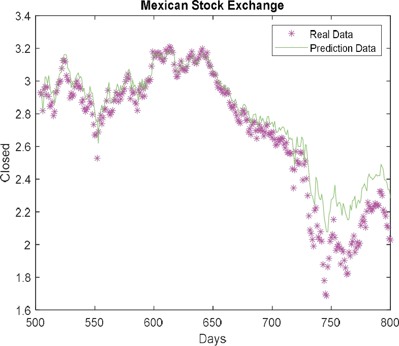
Fig. 11 Plot of real data against predicted data for the type-1 fuzzy system of MSE

Table 8 and Figure 12 illustrates the prediction of the time series using the IT2FS for the Mexican Stock Exchange time series.

Table 8 Results of type-2 FS of MS

Test	Prediction Error 0.3 Uncertainty	Prediction Error 0.4 Uncertainty	Prediction Error 0.5 Uncertainty
1	0.3122	0.2815	0.2512
2	0.3321	0.3017	0.2906
3	0.4256	0.3792	0.4326
4	0.3689	0.3512	0.3891
5	0.5995	0.5725	0.5519
6	0.4912	0.4315	0.4654
7	0.5276	0.5045	0.5618
8	0.3044	0.3426	0.3725
9	0.5122	0.5389	0.5554
10	0.5572	0.5437	0.5215

Fig. 12 Plot of the real data against predicted data for the T2FS

Table 9 shows the results of the genetic algorithm, where the best architecture of the ERNN is shown in row number 2 of Table 9 for the Dow Jones time series.

Table 9 Genetic algorithm results for the RNN for the DJ

Evolutions	Gen.	Ind.	Pm	Pc	Num. Modules	Num. Layers	Num. Neurons	Duration	Prediction Error
1	100	100	0.07	0.6	5	3	24,30,9 13,26,15 17,22,25 13,25,30 1,21,30	18:07:07	0.0023472
2	100	100	0.05	0.7	5	5	5,8,1 12,16,16 9,7,12 6,20,15 1,2,7	16:25:18	0.0018525
3	100	100	0.07	0.5	5	3	22,2,1 14,24,25 9,12,23 8,21,10 1,17,22	17:08:49	0.028711
4	100	100	0.03	0.4	5	2	6,29 6,2 5,17 8,9 2,6	19:09:55	0.0022167
5	100	100	0.09	0.9	5	3	15,16,1 5,10,4 3,16,4 6,30,6 7,30,30	18:05:13	0.0021315
6	100	100	0.05	0.5	5	3	30,11,4 30,18,17 13,9,29 7,21,5 2,1,14	17:20:12	0.0026022
7	100	100	0.09	0.9	5	3	8,1,15 6,22,11 4,8,22 6,30,27 1,10,2	17:22:17	0.0025405
8	100	100	0.09	1	5	3	7,8,1 6,30,6 15,30,8 12,30.27,3 3,30,30	18:23:24	0.0022419
9	100	100	0.04	0.7	5	3	9,9,26 9,15,22 13,28,8 1,19,4 2,10,24	19:20:14	0.002269
10	100	100	0.03	0.7	4	3	16,16,1 4,15,4 6,27,7 10,30,20 17,22,29	19:02:31	0.002593

Table 10 shows the results of the integration type-1 FS for the optimized ERNN, where the result obtained is of experiment number 5, with a prediction error: 0.10567 and Figure 13 represents the plot of real data against predicted data for the type-1 fuzzy system.

Table 10 Results of type-1 FS of DJ

Test	Prediction Error with Type-1 Fuzzy Integration
1	0.11343
2	0.12376
3	0.26920
4	0.14675
5	0.10567
6	0.22561
7	0.17888
8	0.18886
9	0.26922
10

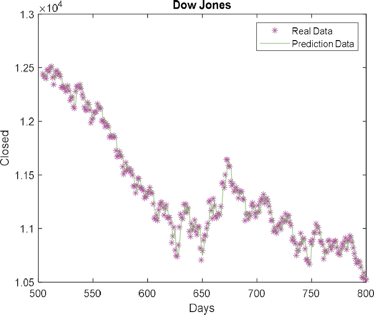
Fig. 13 Plot of real data against predicted data for the type-1 fuzzy system of DJ

Table 11 and Figure 14 represent the prediction of the time series using the IT2FS for the Dow Jones time series.

Table 11 Results of type-2 FS of DJ

Test	Prediction Error 0.3 Uncertainty	Prediction Error 0.4 Uncertainty	Prediction Error 0.5 Uncertainty
1	0.0188	0.0188	0.0172
2	0.0117	0.0117	0.0145
3	0.0156	0.0156	0.0164
4	0.0138	0.0176	0.0137
5	0.0178	0.018	0.0185
6	0.0217	0.0224	0.0243
7	0.0169	0.017	0.0152
8	0.0163	0.0163	0.0165
9	0.0156	0.0154	0.0151
10	0.0208	0.0208	0.0218

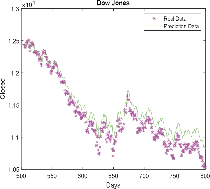
Fig. 14 graph of real data against predicted data for the T2FS of DJ

Table 12 shows the results of the genetic algorithm, where the best architecture of the ERNN is shown in row number 4 of Table 12, for the US/Dollar Mexican Pesos time series.

Table 12 Genetic algorithm results for the RNN of Dollar

Evolutions	Gen.	Ind.	Pm	Pc	Num. Modules	Num. Layers	Num. Neurons	Duration	Prediction Error
1	100	100	0.07	0.6	5	1	1 1 9 6 1	02:01:34	0.00213
2	100	100	0.05	0.7	5	3	11,26,30 4,23,14 1,2,13 12,2,6 1,16,30	07:35:18	0.0018864
3	100	100	0.07	0.5	5	1	1 1 3 11 1	02:21:04	0.0029528
4	100	100	0.03	0.4	5	1	3 6 2 19 3	02:09:55	0.0018685
5	100	100	0.09	0.9	5	1	1 1 1 6 1	02:12:04	0.0030438
6	100	100	0.05	0.5	5	5	5,25,24 7,24,9 1,29,22 4,25,30 1,23,13	02:53:46	0.0020584
7	100	100	0.09	0.8	5	1	2 13 4 6 2	01:54:24	0.0021801
8	100	100	0.09	1	5	1	1 1 1 7 1	01:34:18	0.0021431
9	100	100	0.04	0.7	5	1	1 1 1 2 1	01:38:38	0.0022053
10	100	100	0.03	0.7	5	1	2 12 5 8 1	01:36:38	0.0025446

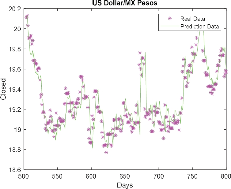
Table 13 illustrates the results of the type-1 FS integration for the optimized ERNN, where the result obtained is of experiment number 4, with a prediction error: 0.113072 and Figure 15 represents the plot of real data against predicted data for the type-1 fuzzy system, for the US/Dollar Mexican Pesos time series.

Table 13 Results of type-1 FS of Dollar data

Test	Prediction Error with Type-1 Fuzzy Integration
1	0.114981
2	0.11307
3	0.115
4	0.113072
5	0.114809
6	0.11319
7	0.119767
8	0.115691
9	0.113076
10	0.114352

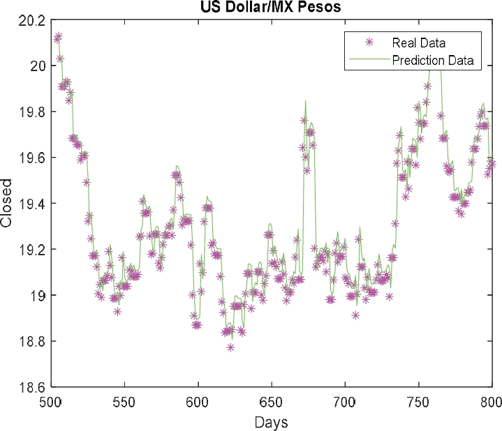
Fig. 15 Plot of real data against predicted data for the type-1 fuzzy system of Dollar

Table 14 and Figure 16 illustrate the prediction of the time series using the IT2FS for the US/Dollar Mexican Pesos time series.

Table 14 Results of type-2 FS of Dollar data

Test	Prediction Error 0.3 Uncertainty	Prediction Error 0.4 Uncertainty	Prediction Error 0.5 Uncertainty
1	0.2341	0.2215	0.3972
2	0.2217	0.2056	0.3779
3	0.2118	0.2019	0.3888
4	0.1979	0.1845	0.3985
5	0.1722	0.1944	0.3612
6	0.1922	0.2251	0.3758
7	0.2012	0.2252	0.3763
8	0.2212	0.2019	0.3794
9	0.2132	0.2313	0.3590
10	0.2055	0.1903	0.3674

Fig. 16 Plot of real data against predicted data for the T2FS of Dollar data

4.1 Comparison of Results

Comparisons were made with the paper called: “A New Method for Type-2 Fuzzy Integration in Ensemble Neural Networks Based on Genetic Algorithms”, where the same data from the series of the Mackey-Glass were used.

In this case, we obtained that recurrent neural networks are better for predicting data from this series since there is a significant difference in the results, as they are better with the recurrent neural than with ensemble neural network.

Therefore, we use a significance of 90% and according to the results obtained and we can say that there is significant improvement with the ensemble neural network, as is summarized in Table 15. Comparisons were also made with the paper called: “Particle swarm optimization of ensemble neural networks with fuzzy aggregation for time series prediction of the Mexican Stock Exchange”, where the same data from the series of the Mexican stock exchange were used.

Table 15 Results of comparison of the Mackey-Glass

Time Series	N(RNN)	N(ENN)	Value(T)	Value(P)
Dow Jones	30	30	-0.5091	0.0694

We obtained that recurrent neural network is better for predicting data from this series since there is a significant difference in the results are better the recurrent neural that with ensemble neural network. Therefore, we use a significance of 99% and according to the results obtained we can say that there is significant improvement with the ensemble neural network, as summarizes in Table 16.

Table 16 Results of comparison of the Mexican Stock Exchange

Time Series	N(RNN)	N(ENN)	Value(T)	Value(P)
Mexican Stock Exchange	30	30	-9.0370	0.000

Comparisons were made with the paper called: “Optimization of Ensemble Neural Networks with Type-2 Fuzzy Integration of Responses for the Dow Jones Time Series Prediction”, where the same data from the series of the Dow Jones were used and we obtained that recurrent neural networks are better for predicting data from this series since there is a no significant difference in the results are better the recurrent neural that with ensemble neural network.

Therefore, we use a significance of 90% and according to the results obtained we can say that there is significant improvement with the ensemble neural network, as is summarized in Table 17.

Table 17 Results of comparison of the Dow Jones

Time Series	N(RNN)	N(ENN)	Value(T)	Value(P)
Mackey-Glass	30	30	1.3732	0.090

5 Conclusions

In this work the design, implementation, and optimization of ensemble recurrent neural network for the prediction time are presented.

The chosen algorithm for this optimization was the GA, with which a total of 30 different experiments were made.

Comparisons were made with previously carried out works, in this way it can be said that genetic algorithms are an optimization technique that gives good results for the forecast of the time series. The main contribution in this paper was the creation of the new model of recurrent neural networks presented in this document that has shown good results since they are effective for the prediction of time series.

A hierarchical GA was applied to optimize the architecture of the RNN, in terms of parameters (NM, NL NN), to find better architecture and the time series error. The integration of the network responses was done with a type-1 and T2FS, to obtain the prediction error of the proposed time series, such as Mackey Glass benchmark, Mexican Stock Exchange, Dow Jones, and Exchange Rate of US Dollar/Mexican Pesos time series.

Analyzing the results, we can say that the combination of these intelligent computing techniques generates excellent results for this type of problem since the recurrent neural networks analyze the data of time series, the Genetic algorithms perform optimization and they helped us find the best architecture of the RNN, as well as to obtain the best solution to the proposed problem.

As future work we plan to perform optimization of the recurrent neural network with another optimization method, and make comparisons of the type-1 and type-2 fuzzy systems. We will also consider other complex time series to test the ability of our method for predicting complex time series.

Acknowledgments

We would like to express our gratitude to the CONACYT and Tijuana Institute of Technology for the facilities and resources granted for the development of this research.

References

1. Apaydin, H., Feizi, H., Sattari, M. T., Colak, M. S., Shamshirband, S., Chau, K. W. (2020). Comparative analysis of recurrent neural network architectures for reservoir inflow forecasting. Water, Vol. 12, No. 5, pp. 1–18, DOI: 10.3390/w12051500. [ Links ]

2. Chang, B., Chen, M., Haber, E., Chi, E. H. (2019). Antisymmetric RNN: A dynamical system view on recurrent neural networks. International Conference on Learning Representations, pp. 2–6. DOI: 10.48550/arXiv.1902.09689. [ Links ]

3. Brockwell, P. D., Davis, R. A. (2002). Introduction to time series and forecasting. Springer-Verlag, New York, pp. 259316. DOI: 10.1007/0-387-21657-X_8. [ Links ]

4. Castillo, O., Hidalgo, D., Cervantes, L., Melin, P., Martínez, R. (2020). Fuzzy parameter adaptation in genetic algorithms for the optimization of fuzzy integrators in modular neural networks for multimodal biometry. Computación y Sistemas, Vol. 24 No. 3, pp. 1093–1105. DOI: 10.13053/cys-24-3-3329. [ Links ]

5. Castillo, O., Amador-Angulo, L. (2018). Generalized type-2 fuzzy logic approach for dynamic parameter adaptation in bee colony optimization applied to fuzzy controller design. Information Sciences, Vol. 460-461, pp. 476–496. DOI: 10.1016/j.ins.2017.10.032. [ Links ]

6. Castillo, O., Melin, P. (2007). Comparison of hybrid intelligent systems neural networks and interval type-2 fuzzy logic for time series prediction. Proceedings IJCNN 2007, pp. 3086–3091. DOI: 10.1109/IJCNN.2007.4371453. [ Links ]

7. Castillo, O., Melin, P. (2002). Hybrid intelligent systems for time series prediction using neural networks, fuzzy logic, and fractal theory. Neural Networks, IEEE Transactions on, Vol. 13, No. 6. pp. 1395–1408. DOI: 10.1109/TNN.2002.804316. [ Links ]

8. Castillo, O., Melin, P. (2001). Simulation and forecasting complex economic time series using neural networks and fuzzy logic. Proceedings of the International Neural Networks Conference Vol. 3, pp. 1805–1810. DOI: 10.1109/IJCNN.2001.938436. [ Links ]

9. Castillo, O., Melin, P. (2001). Simulation and forecasting complex financial time series using neural networks and fuzzy logic. Proceedings the IEEE the International Conference on Systems, Man and Cybernetics Vol. 4, pp. 2664–2669. DOI: 10.1109/ICSMC. 2001.972967. [ Links ]

10. Castillo, O., Melin, P. (2008). Type-2 fuzzy systems, type-2 fuzzy logic theory and application. Springer, pp. 30–43. DOI: 10.1109/GrC.2007.118. [ Links ]

11. Castillo, O., Melin, P. (2007). Comparison of hybrid intelligent systems, neural networks and interval type-2 fuzzy logic for time series prediction. Proceedings IJCNN, pp. 3086–3091. DOI: 10.1109/IJCNN.2007. 4371453. [ Links ]

12. Castro, J. R., Castillo, O., Melin, P., Mendoza, O., Rodríguez-Díaz, A. (2011). An interval type-2 fuzzy neural network for chaotic time series prediction with cross-validation and akaike test. Soft Computing for Intelligent Control and Robotics, Vol. 318, pp. 269–285. DOI: 10.1007/978-3-642-15534-5_17. [ Links ]

13. Smith, C., Jin, Y. (2014). Evolutionary multi-objective generation of recurrent neural network ensembles for time series prediction. Neurocomputing, Vol. 143, pp. 1–10. DOI: /10.1016/j.neucom.2014.05.062. [ Links ]

14. Cowpertwait, P., Metcalfe, A. (2009). Time series, introductory time series with R. Springer Dordrecht Heidelberg London New York, pp. 2–5. [ Links ]

15. Dow Jones Company. (2021). https://www.dowjones.com. [ Links ]

16. Fekri, M. N., Patel, H., Grolinger, K., Sharma, V. (2021). Deep learning for load forecasting with smart meter data: Online adaptive recurrent neural network. Applied Energy, Vol. 282, pp. 1–17, DOI: 10.1016/j.apenergy.2020.116177. [ Links ]

17. Gaxiola, F., Melin, P., Valdez, F., Castillo, O. (2014). Interval type-2 fuzzy weight adjustment for backpropagation neural networks with application in time series prediction. Information Sciences Vol. 260, No. 1, pp. 1–14. DOI: 10.1016/j.ins.2013.11.006. [ Links ]

18. Goldberg, D. (1989). Genetic algorithms in search, optimization and machine learning. Addison Wesley. [ Links ]

19. Hewamalage, H., Bergmeir, C., Bandara, K. (2021). Recurrent neural networks for time series forecasting: current status and future directions. Vol. 37, No. 1, pp. 388–427. DOI: 10.1016/j.ijforecast.2020.06.008. [ Links ]

20. Triebe, O., Hewamalage, H., Pilyugina, P., Laptev, N., Bergmeir, C., Rajagopal, R. (2021). Neuralprophet: explainable forecasting at scale. arXiv:2111.15397. [ Links ]

21. Jerome, T., Connor, R., Douglas, M. (1994). Recurrent neural networks and robust time series Prediction, IEEE Transactions on Neural Networks, Vol. 5, No. 2, pp. 240–254. DOI: 10.1109/72.279188. [ Links ]

22. Wen, J., Wu, L., Chai, J. (2020). Paper citation count prediction based on recurrent neural network with gated recurrent unit. IEEE 10th International Conference on Electronics Information and Emergency Communication (ICEIEC), pp. 303–306. DOI: 10.1109/ICEIEC49280.2020.9152330. [ Links ]

23. Jilani, T. A., Burney, S. M. A. (2008). A refined fuzzy time series model for stock market forecasting. Physica-A-Statistical mechanics and its applications, Vol. 387, No. 12, pp. 2857–2862. DOI: 10.1016/j.physa.2008.01.099. [ Links ]

24. Wen, J., Wu, L., Chai, J. (2020). Paper citation count prediction based on recurrent neural network with gated recurrent unit. IEEE 10th International Conference on Electronics Information and Emergency Communication (ICEIEC), pp. 303–306. [ Links ]

25. Karnik, N., Mendel, J. M. (1999). Applications of type-2 fuzzy logic systems to forecasting of time-series. Information Sciences, Vol. 120, No. 1–4, pp. 89-111. DOI: 10.1016/S0020-0255(99)00067-5. [ Links ]

26. Karnik, N., Mendel, J. M. (2001). Operations on type-2 set. Fuzzy Set and Systems, Vol. 122, No. 2, pp. 327–348. DOI: 10.1016/S0165-0114(00)00079-8. [ Links ]

27. Lu, S., Zhang, Q., Chen, G., Seng, D. (2021). A combined method for short-term traffic flow prediction based on recurrent neural network. Alexandria Engineering Journal. Vol. 60, No. 1, pp. 87–94, DOI: 10.1016/j.aej.2020.06.008. [ Links ]

28. Mackey, M. C. (2007). Adventures in Poland: having fun and doing research with Andrzej Lasota. Mat. Stosow, pp. 5–32. [ Links ]

29. Mackey, M. C., Glass, L. (1997). Oscillation and chaos in physiological control systems. Science, Vol. 197, No. 4300, pp. 287–289. DOI: 10.1126/science.267326. [ Links ]

30. Man, K., Tang, K., Kwong, S. (1998). Genetic algorithms and designs, introduction, background and biological background. Springer-Verlag London Limited, pp. 1–62. [ Links ]

31. Melin, P., Castillo, O., González, S., Cota, J., Trujillo, W. L., Osuna, P. (2007). Design of modular neural networks with fuzzy integration applied to time series prediction. Springer Berlin / Heidelberg, Vol. 41, pp. 265–273. DOI: 10.1007/978-3-540-72432-2_27. [ Links ]

32. Melin, P., Soto, J., Castillo, O., Soria, J. (2012). A new approach for time series prediction using ensembles of anfis models. Expert Systems with Applications (2011). [ Links ]

33. Mendel, J. (2001). Uncertain rule-based fuzzy logic systems, introduction of new directions. Prentice-Hall, Inc., Vol. 2, No. 1, pp. 72–73. DOI: 10.1109/MCI.2007.357196. [ Links ]

34. Mencattini, A., Salmeri, M. S., Mertazzoni, B., Lojacono, R., Pasero, E., Moniaci, W. (2005). Local meteorological forecasting by type-2 fuzzy systems time series prediction. CIMSA - IEEE International Conference on Computational Intelligence for Measurement Systems and Applications Giardini Naxos, Italy, pp. 20–22. [ Links ]

35. Mexican Bank Database (2021). https://www.banxico.org.mx [ Links ]

36. Min, H., Jianhui, X., Shiguo, X., Fu-Liang, Y. (2004). Pred of chaotic time series based on the recurrent predictor neural network. IEEE, Vol. 52, No. 12, pp. 3409–3416, DOI: 10.1109/TSP.2004.837418. [ Links ]

37. Mikolov, T., Kombrink, S., Burget, L., Černocký, J., Khudanpur, S. (2011). Extensions of recurrent neural network language model. IEEE International Conference on Acoustics, Speech and Signal Processing (ICASSP), pp. 552–5531. DOI: 10.1109/ICASSP.2011.5947611. [ Links ]

38. Olivas, F., Valdez, F., Melin, P., Sombra, A., Castillo, O. (2019). Interval type-2 fuzzy logic for dynamic parameter adaptation in a modified gravitational search algorithm. Information Sciences Vol. 476, pp. 159–175. [ Links ]

39. Pang, Z., Niu, F., O’Neill, Z. (2020). Solar radiation prediction using recurrent neural network and artificial neural network: A case study with comparisons. Renewable Energy, Vol. 156, pp. 279–289. DOI: 10.1016/j.renene.2020.04.042. [ Links ]

40. Valdez, F., Castillo, O., Peraza, C. (2020). Fuzzy logic in dynamic parameter adaptation of harmony search optimization for benchmark functions and fuzzy controller. International Journal of Fuzzy Systems, Vol. 22, pp. 1198–1211 DOI: 10.1007/s40815-020-00860-7. [ Links ]

41. Petnehazi, G. (2019). Recurrent neural networks for time series forecasting. University of Debrecen, pp. 1–22. [ Links ]

42. Pulido, M., Melin, P. (2021). Ensemble recurrent neural networks for complex time series prediction with integration methods, Fuzzy logic hybrid extensions of neural and optimization algorithms theory and applications. Studies in Computational Intelligence, Vol 940, pp. 71–83 DOI: 10.1007/978-3-030-68776-2_4 pp. 71-83. [ Links ]

43. Pulido, M., Mancilla, A., Melin, P. (2009). An ensemble neural network architecture with fuzzy response integration for complex time series prediction. In: Castillo, O., Pedrycz, W., Kacprzyk, J., editors, Evolutionary Design of Intelligent Systems in Modeling, Simulation and Control. Studies in Computational Intelligence, Springer, Berlin, Heidelberg. Vol 257. 85–110. DOI: 10.1007/978-3-642-04514-1_6. [ Links ]

44. Pulido, M., Melin, P., Castillo, O. (2014). Particle swarm optimization of ensemble neural networks with fuzzy aggregation for time series prediction of the Mexican Stock Exchange. Information Sciences, Vol. 208, pp. 188–204. DOI: 10.1016/j.ins.2014.05.006. [ Links ]

45. Melin, P., Pulido, M. (2014). Optimization of ensemble neural networks with type-2 fuzzy integration of responses for the dow jones time series prediction. Intelligent Automation & Soft Computing, Vol. 20, No. 3, pp, 403–418. DOI: 10.1080/10798587.2014.893047. [ Links ]

46. Pulido, M., Melin, P. (2021). Comparison of genetic algorithm and particle swarm optimization of ensemble neural networks for complex time series prediction. In: Melin, P., Castillo, O., Kacprzyk, J., editors, Recent Advances of Hybrid Intelligent Systems Based on Soft Computing. Studies in Computational Intelligence, Vol 915. Springer, Cham. DOI: 10.1007/978-3-030-58728-4_3. [ Links ]

47. Rohitash, C., Mengjie, Z. (2012). Cooperative coevolution of Elman recurrent neural networks for chaotic time series Prediction. Neurocomputing, Vol. 86, pp. 116–123. DOI: 10.1016/j.neucom.2012.01.014. [ Links ]

48. Sharkey, A. J. C. (1999). Combining artificial neural nets: ensemble and modular multi-net systems. Perspectives in Neural Computing, Springer-Verlag, London. [ Links ]

49. Sharkey, A. J. C. (1996). One combining artificial of neural nets. Department of Computer Science University of Sheffield, U.K. Vol. 8, No. 3-4, DOI: 10.1080/095400996116785. [ Links ]

50. Sherstinsky, A. (2020). Fundamentals of recurrent neural network (rnn) and long short-term memory (lstm) network. Physica D: Nonlinear Phenomena, Vol. 404, pp.1–28. DOI: 10.1016/j.physd.2019.132306. [ Links ]

51. Slawek, S. (2020). A hybrid method of exponential smoothing and recurrent neural networks for time series forecasting. International Journal of Forecasting, Vol. 36, No. 1, pp. 75–85. DOI: 10.1016/j.ijforecast.2019.03.017. [ Links ]

52. Sollich, P., Krogh, A. (1996). Learning with ensembles: how over-fitting can be useful, D. S., Touretzky, M. C., Mozer, M. E., Hasselmo (Eds.), Advances in Neural Information Processing Systems 8, Denver, CO, MIT Press, Cambridge, MA, pp.190–196. [ Links ]

53. Soto, J., Melin, P., Castillo, O. (2018). A new approach for time series prediction using ensembles of it2fnn models with optimization of fuzzy integrators. International Journal of Fuzzy Systems, Vol. 20, pp. 701–728. DOI: 10.1007/s40815-017-0443-6. [ Links ]

54. Soto, J., Melin, P., Castillo, O. (2014). Time series prediction using ensembles of ANFIS models with genetic optimization of interval type-2 and type-1 fuzzy integrators. International Journal of Hybrid Intelligent system Vol. 11, No. 3, pp. 211–226. DOI: 10.3233/HIS-140196. [ Links ]

55. Sudipto, S., Raghava, G. P. S. (2006). Prediction of continuous B-cell epitopes in an antigen using recurrent neural network. National Library of Medicine, Vol. 65, No. 1, pp. 40–48. DOI: 10.1002/prot.21078 [ Links ]

56. Walid, A. (2016). Recurrent neural network for forecasting time series with long memory pattern. Journal of Physics: Conference Series, Vol. 824, pp. 1–8. DOI: 10.1088/1742-6596/824/1/012038. [ Links ]

57. Wei, X., Zhan, L., Yang, H. Q., Zhang, L., Yao, Y. P. (2020). Machine learning for pore-water pressure time-series prediction: Application of recurrent neural networks, Geoscience Frontiers, Vol. 12, No. 1, pp. 453–467. DOI: 10.1016/j.gsf.2020.04.011. [ Links ]

58. Whitley, L. D. (2017). Foundations of genetic algorithms 2. Morgan Kaufman Publishers (1993), pp. 332. [ Links ]

59. Yao, Q., Dongjin, S., Haifeng, C., Wei, C., Guofei, J., Garrison, C. (2017). A dual-stage attention-based recurrent neural network for time series prediction. Computer science, Cornell University, pp. 1–7. [ Links ]

60. Zadeh, L. A. (1965). Fuzzy sets. Information and control. Vol. 8, pp. 338–353. [ Links ]

61. Zhan, J., Man, K. F. (1998). Time series Prediction using recurrent neural network in multi-dimension embedding phase space. IEEE International Conference on Systems, Man and Cybernetics, Vol. 2 pp. 1868–1873 DOI: 10.1109/ICSMC.1998.728168. [ Links ]

62. Zhang, D., Peng, Q., Lin, J., Wang, D., Liu, X., Zhuang, J. (2019). Simulating reservoir operation using a recurrent neural network algorithm. Water, Vol. 11 No. 4, pp. 1–18, DOI: 10.3390/w11040865. [ Links ]

63. Zhang, J. S., Xio, X. C. (2000). Predicting chaotic time series using recurrent neural network. Published under licence by IOP Publishing Ltd, pp. 88–90. [ Links ]

64. Zhou, Y., Guo, S., Xu, C.Y., Chang, F.J., Yin, J. (2020). Improving the reliability of probabilistic multi-step-ahead flood forecasting by fusing unscented Kalman filter with recurrent neural network. Water, Vol. 12, No. 2, pp. 1–15, DOI: 10.3390/w12020578. [ Links ]

Received: June 10, 2021; Accepted: November 16, 2021

^* Corresponding author: Patricia Melin, e-mail: pmelin@tectijuana.mx

This is an open-access article distributed under the terms of the Creative Commons Attribution License